MATH213: Advanced Mathematics for Software Engineers

Taken in Winter 2024. Taught by Dr. Matthew Harris. Office EIT 4018.

Course Description: Laplace transform methods for: solving linear ordinary differential equations, classical signals, and systems. Transfer functions, poles, and zeros; system stability. Frequency response of linear systems and its log-scale representation (Bode plot). Fourier series. Applications in areas of interest for software engineers and computer scientists. Brief introduction to Fourier transforms in the context of signals and systems.

Course website: https://ece.uwaterloo.ca/~math213/index.html. But everything is on Learn.

Final

• Laplace transform
• Fourier transform
• Here is a Fourier series, use it to find a fourier of another thing
• Integration tricks
• If functions converges
• Difficulty level of homework (tutorial)
• Can also ask Laplace stuff
• True and false questions
• Mostly computations, linear : is it causal,, etc.

Final Study MATH213

Midterm

https://tutorial.math.lamar.edu/Classes/DE/LaplaceIntro.aspx

Review:

• Partial Fraction integrals
• Integration by parts
• Lecture 1 and 2
• Lecture 3 and 4
• Lecture 5
• Lecture 6
• Lecture 7
• Lecture 8
• Lecture 9
• Lecture 10
• Lecture 11 - midterm review
• All tutorials
• Properties of Laplace transform

Midterm MATH213

Messed up entirely on the question asking us to perform Convolution Theorem. Instead did it by definition…

Concepts

• Differential Equations
• Ordinary Differential Equations
• Laplace Transform
• Inverse Laplace Transform
• Laplace Table
• Convolution
• Initial Value Theorem
• Transfer Function
• Final Value Theorem
• Signal
• Bifurcation Diagram
• Fourier Series

A5: Up to Lecture 18? L19 helps with drawing plots and Q4c-d (which are quick after you have the results from a-b) need results from L19 to complete. That said if you think about what the plots mean you can likely work out the needed results pretty quickly.

Lecture 1

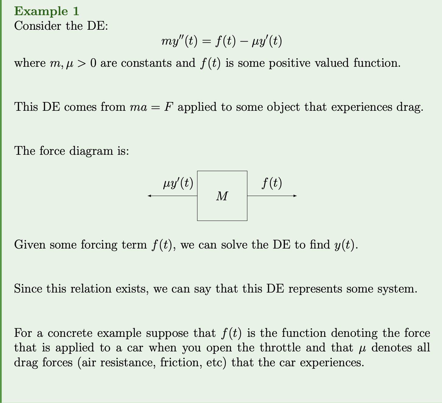
What are DEs and where do they come from?

Isaac Newton

Introduction to Differential Equations DEs.

Not so sure about Example 6. Very confusing

Lecture 2

Definition 1: Independent and Dependent Variables and Parameters

The dependent variable(s) of a DE are the unknown functions that we want to solve for i.e. $f(x),y(x,t),$ etc.

The independent variable(s) of a DE are the variable(s) that the independent variable(s) depend on i.e. $x,t,$ etc.

A parameter is a term that is an unknown but is not an independent or dependent variable i.e $a,b,\alpha ,\beta ,$ etc.

Definition 2: Order of a DE

The order of a DE is the order of the highest derivative.

Definition 3: ODEs and PDEs

A DE is an ordinary differential equation (ODE) if it only contains ordinary derivatives (i.e. no partial derivatives)

A DE is a partial differential equation (PDE) if it contains at least one partial derivative of a independent variable.

Definition 4: Linear and nonlinear DEs

A DE that contains no products of terms involving the dependent variable(s) is called linear.

If a DE is not linear then it is nonlinear.

Definition 5: Homogeneous and Inhomogeneous: DEs

DE where every term depends on a dependent variable is called homogeneous.

A DE that is not homogeneous is called inhomogeneous or nonhomogeneous.

Linear homogeneous DEs have the property that if $f_1$ and $f_2$ both solve the DE then so does $a{f}_1+b{f}_2$ for all$a,b\in \mathbb{R}$.

This is the same property that was used to define linearity in MATH115! i.e. a vector valued function $f:{\mathbb{R}}^n\to {\mathbb{R}}^m$ is linear if and only if for all $\vec{x},\vec{y}\in {\mathbb{R}}^n$ and for all $a,b,\in \mathbb{R},f(a\vec{x}+b\vec{y})=af(\vec{x})+bf(\vec{y})$.

The difference is that we now study linear functions applied to the vector space of all sufficiently differentiable functions (e.g. $C^{\infty }(\mathbb{R})$) instead of vectors in ${\mathbb{R}}^n$ i.e. there are no matrix representations for linear functions.

Theorem 1: Linear ODEs with Variable Coefficients

All ODEs of the form $\frac{d^n}{d{t}^n}y(t)+a_{n-1}(t)\frac{d^{n-1}}{d{t}^{n-1}}y(t)+...+a_0(t)y(t)=f(t)$ where $n\in 0,1,...,n$, the $a_i(t)$ functions are real valued, but $y(t)$ and $f(t)$ can be complex valued are linear ODEs.

Here $f(t)$ is called the forcing term.

Lecture 3

Laplace Transform Motivation:

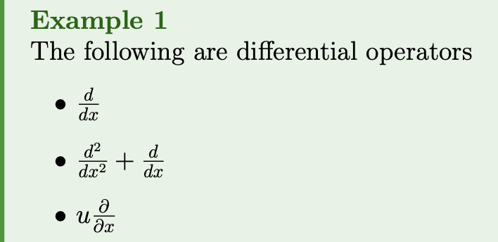
Definition 1: Differential operator

A differential operator is a special type of function (called a functional) that accepts a function and returns another function and only consists of taking derivatives, multiplying by functions, and adding other differential operators.

Example:

All ODEs are of the form:

$$D(y(x))=g(x)$$

where $y$ is the dependent variable, $x$ is the independent variable, $g(x)$ is the forcing term and $D$ is a differential operator.

Also in MATH115 we studied functionals called linear transformations!

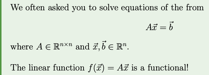
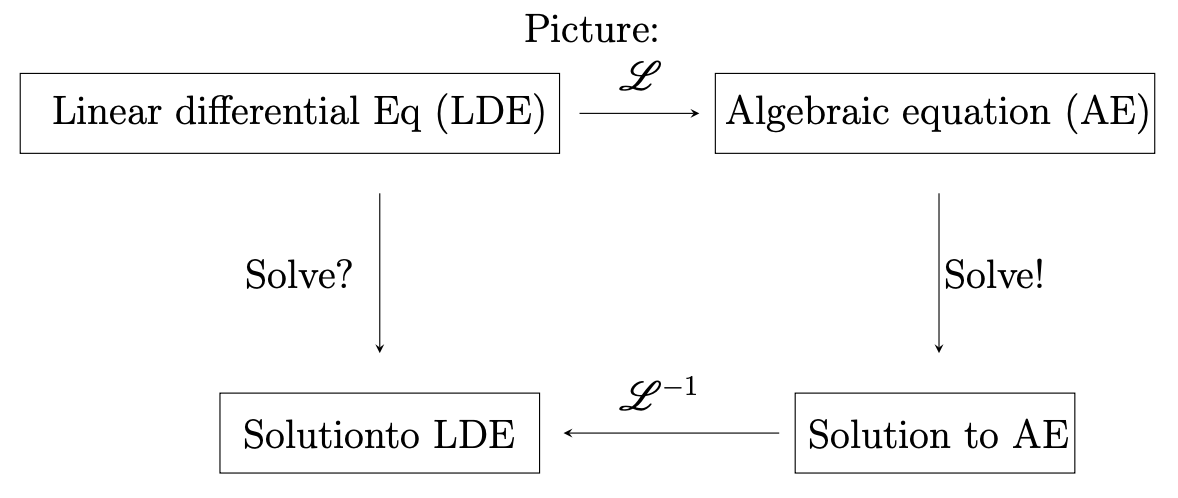
Note: $A\vec{x}=\vec{b}$ looks quite similar to $Dy=g$ given that $D$ is linear …

This is the basis of the Laplace transform approach to solving ODEs.

Laplace Transform and Inverse Laplace Transform

Lecture 4

Lecture goal:

• be able to compute Laplace transforms from the definition
• know what one-sided or unilateral Laplace Transform is
• understand some commonly used (and important) properties of the Laplace transform

Definition 1: Unilateral Laplace Transform

The Unilateral Laplace Transform or One-sided Laplace Transform of a function $f(t)$ defined only for $t\ge 0$ is defined as $F(s)=\mathcal{L}\{f(t)\}={\int }_{O^{+}}^{\infty }f(t)e^{-st}dt$

Caution: If we use the symbol "$\mathcal{L}$" we mean the two sided transform unless otherwise stated.

Bunch of examples. Go see.

Properties of the Laplace Transform:

Theorem 1

For any function $f(t)$, the one-sided Laplace transform will always converge given that there is some sufficiently large $s\in \mathbb{R}$ such that ${\int }_0^{\infty }f(t)e^{-st}dt$ exists

Theorem 2: Laplace Transform is Linear

Suppose that $f(t)$ and $g(t)$ have Laplace transform $F(s)$ and $G(s)$.

Then for all $\alpha ,\beta \in C$ $\mathcal{L}${$\alpha f(t)+\beta g(t)$} $=\alpha F(s)+\beta G(s)$ the ROC is the intersection of the ROCs for $F(s)$ and $G(s)$.

Theorem 3: Time-Scaling

If $\mathcal{L}${$f(t)$}$=F(s)$ then for $c>0,\mathcal{L}${$f(ct)$}$=\frac{1}{c}F(\frac{s}{c})$

Theorem 4: Exponential Modulation

$\mathcal{L}\{e^{\alpha t}f(t)\}=F(s-\alpha )$

Prof said he might ask proofs in exams.

Theorem 5: Time-Shifting

If $F(s)=\mathcal{L}\{f(t)u(t)\}$ and $g(t)=f(t-T)u(t-T)$ then $G(s)=e^{-sT}F(s)$.

Theorem 6: Multiplication by t

If $\mathcal{L}\{f(t)\}=F(s)$ then $\mathcal{L}\{tf(t)\}=-\frac{d}{ds}F(s)$.

Theorem 7: Laplace Transform of a Derivative / Integral

Let $f(t)$ be such that there is a real value $\alpha$ such that the integral ${\int }_{0^{+}}^{\infty }|f(t)|e^{-\alpha t}dt$ converge and such that there exists a function $f^{\prime }(t)$ such that for $t\ge 0$ $f(t)=f(0^{+})+{\int }_{0^{+}}^{\infty }{f}^{\prime }(t)d\tau$ and there exists a real value $\beta$ such that ${\int }_{O^{+}}^{\infty }|f^{\prime }(t)|e^{-\beta t}dt$ converges. In this case $F(s)=\frac{1}{s}f(O^{+})+\frac{1}{s}\mathcal{L}\{f^{\prime }(t)\}$ or in other-words $\mathcal{L}\{f^{\prime }(t)\}=sF(s)-f(0^{+})$

The proof for this is basically in the previous example. Example 8. This theorem is how we will solve linear DEs!!!

Lecture 5

Lecture goals:

• know how to use Laplace Transform table and the properties of the Laplace transform to evaluate Laplace Transforms and “simple” inverse Laplace Transforms.
• know what the convolution operator is and its connection to Laplace Transforms

2 pretty straightforward examples.

Convolution

Before solving DEs we introduce one more super useful property of the Laplace Transform by first introducing convolution.

To motivate the continuous convolution operator we start with some discrete cases.

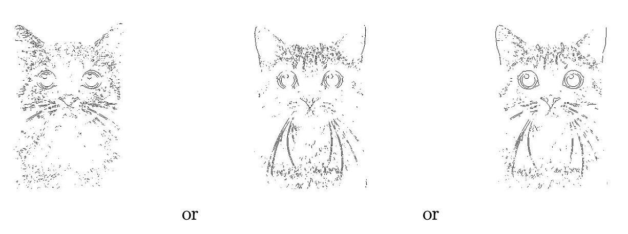
2D Image filtering: Consider the image of a random internet cat:

Suppose we wanted to blur the image. We could do this by replacing each pixel with a weighted average of the nearby pixels

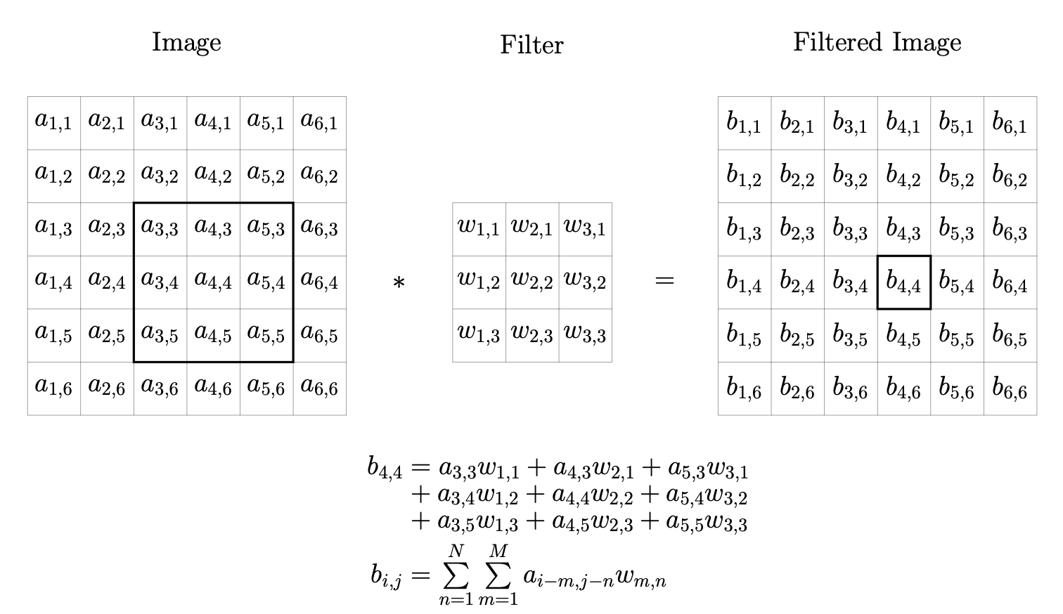
This process of filtering the image is called discrete convolution. If we use a Gaussian filter matrix i.e. something of the form:

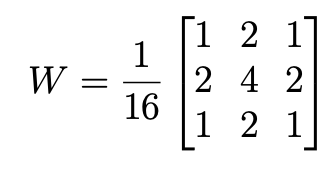
then the filtered cat image becomes

If we use a Sobel filter matrix i.e. something of the form

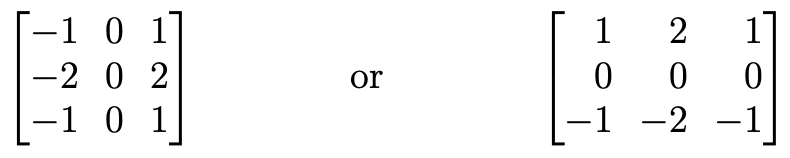
or the norm of the results then the aforementioned filtered cat images are summed becomes

Polynomial Multiplication:

Suppose that $p(x)=a_0+a_{1}x+...+a_m{x}^m$ and $q(x)=b_0+b_{1}x+...+b_n{x}^n$. The product would be

$$p(x)q(x)=a_0{b}_0+(a_1{b}_0+a_0{b}_1)x+(a_2{b}_0+a_1{b}_1+a_0{b}_2)x^2+...+a_m{b}_n{a}^{n+m}$$

Note that the coefficient of $x^i$ is just

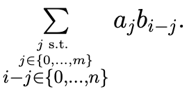
This has the same functional form as the filtering example (but is in 1D) and hence a 1D convolution of the vectors $[a_0,...,a_m]$ and $[b_0,...,b_n]$.

Continuous Convolution:

Motivated by the previous discrete applications we define a continuous version of the convolution.

Definition 1: Convolution

The convolution of the functions $f(t)$ and $g(t)$, denoted by $(f\ast g)(t)$ is the integral $(f\ast g)(t)={\int }_{-\infty }^{\infty }f(\tau )g(t-\tau )d\tau$ given that the integral converges.

Before we continue, we define the idea

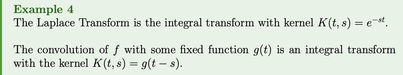
Definition 2: Integral Transform

An integral transform is a functional (function on a set of functions) that can be written in the form

$\mathcal{T}\{f(t)\}={\int }_{-\infty }^{\infty }f(t)K(t,s)dt$.

The function $K(t,u)$ is called the kernel of the integral transform.

Convolution Properties:

Theorem 1: Convolution Properties

A. The convolution operator is commutative $(f\ast g)(t)=(g\ast f)(t)$ B. If $f(t)$ and $g(t)$ are one-sided functions (i.e. $f(t)=g(t)=0$ for $t<0$) then

$(f\ast g)(t)={\int }_0^{t}f(\tau )g(t-\tau )d\tau$

and hence the convolution is also one sided.

Theorem 2: Convolution Theorem

If there exists $\alpha ,\beta \in \mathbb{R}$ such that the integrals

${\int }_{-\infty }^{\infty }|f(t)|e^{-\alpha t}dt$

and

${\int }_{-\infty }^{\infty }|g(t)|e^{-\beta t}dt$

converge then,

$\mathcal{L}\{(f\ast g)(t)\}=F(s)G(s)$

This theorem states that the Laplace Transform of a convolution is the product of the transforms! A direct result of this allows us to “quickly” compute inverse Laplace transforms:

$$\mathcal{L}\{F(s)G(s)\}=(f\ast g)(t)$$

Note: for real valued functions $f$ and $g$, the convolution is a real valued integral (i.e. not a contour integral in the complex plane)!

Lecture 6 - Solving DEs via Laplace Transforms

Definition 1: Characteristic Polynomial

The Characteristic Polynomial of a linear differential equation with constant coefficients

$\frac{d^n}{d{t}^n}y(t)+a_{n-1}\frac{d^{n-1}}{d{t}^{n-1}}y(t)+..+a_{0}y(t)=f(t)$

The polynomial multiplied by $Y(s)$ after you take the Laplace transform. This polynomial will always be $p(s)=s^n+a_{n-1}{s}^{n-1}+...+a_0$

4 examples: need to be able to do the Partial Fractions. I understand but still need to do example 4 PF as exercise.

Extensions of our method: Our method also “works” for some Linear ODEs with non-constant coefficient. The problems are

1. evaluating the Laplace transform of $a(t)y^{(n)}(t)$ for some given function $a(t)$ and a unknown function $y^{(n)}$ and
2. we end up with another (but simpler) differential equation to solve.

If $a(t)=t^n$ then this is particularly “nice”!

Example 5.

Lecture 7 - Rational Functions, Poles, and Initial and Final Value Theorems

Lecture goals:

• understand what a pole is and
• understand the initial and final value theorems After computing the Laplace transform of a function we usually end up with a function that is the ratio of polynomials. Such functions have a name.

Definition 1: Rational Function

A rational function is a function of the form $\frac{P(x)}{Q(x)}$ where $P(x)$ and $Q(x)$ are polynomials.

Definition 2: Regularization

A function $f$ is the regularization of a function $g$ if

1. For all $x$ in the domain of $g$, $f(x)=g(x)$.
2. For all $x$ such that ${\lim }_{t\to x}(g(x))$ exists but $f(x)$ is undefined, $f(x)={\lim }_{t\to x}g(x)$.

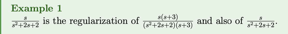
Theorem 1

If $f(x)$ is the regularization of a function $g$ that has a finite number of discontinuities then $\int f(x)dx=\int g(x)dx$.

Definition 3: Finite Zeros and Finite Poles

A rational function $f(x)=\frac{P(x)}{Q(x)}$ that is its own continuous continuation the roots of $P(x)$ are called the **(finite) zeros of ** $f$ and the roots of $Q(x)$ are called the (finite) poles of $f$.

Definition 4: Poles and Zeros at Infinity

Given a rational function $f(x)=\frac{P(x)}{Q(x)}$ has zero at infinity if ${\lim }_{s\to \infty }F(s)=0$. $f(x)$ is said to have a pole at infinity if its reciprocal has a zero at infinity.

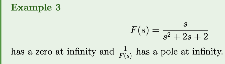
Convention 1: Unless otherwise stated when we talk about poles and zeros we mean the finite poles and finite zeros.

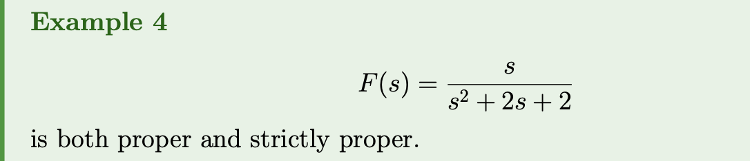
Definition 5: Proper and Strictly Proper Rational Functions

A rational function is proper if the degree of its numerator is less than or equal to that of its denominator. A function is strictly proper if the degree of the numerator is strictly less than that of its denominator.

We care about these ideas because the inverse Laplace transform is a complex valued integral and because of this, we can compute the inverse transform of $F(s)$ by only knowing information about the poles of $F(s)$.

Two important results that are related to poles (and more later).

The initial value theorem:

Definition 6: Piecewise Continuous

A function $f(x)$ is piecewise-continuous on a given finite interval if

1. $f$ has a finite number of discontinuities in that interval and
2. for each discontinuity $x_0$ both the left and right hand limits exits (note they can be different values)

Theorem 2: Initial Value Theorem

If $f(t)$ is a piecewise-continuous and ${\int }_0^{\infty }|f(t)|e^{-\alpha t}$ converges for some $\alpha \in \mathbb{R}$ then

$f(0^{+)=}{\lim }_{s\to +\infty }sF(s)$

Understand this theorem:

• The above gives us a way of computing the IC of $f(t)$ from $F(s)$ without computing the inverse Laplace transform and instead evaluating a limit in the complex plane
• $s$ is generally complex so the limit is in the complex plane NOT the real number line thus:
  • $Re(s)$ tends to infinity
  • $Im(s)$ can do anything (stay 0, oscillate, go to infinity, do random things, etc.)
• For many problems we can treat the limit as the standard limit you are used to working with.

The final value theorem:

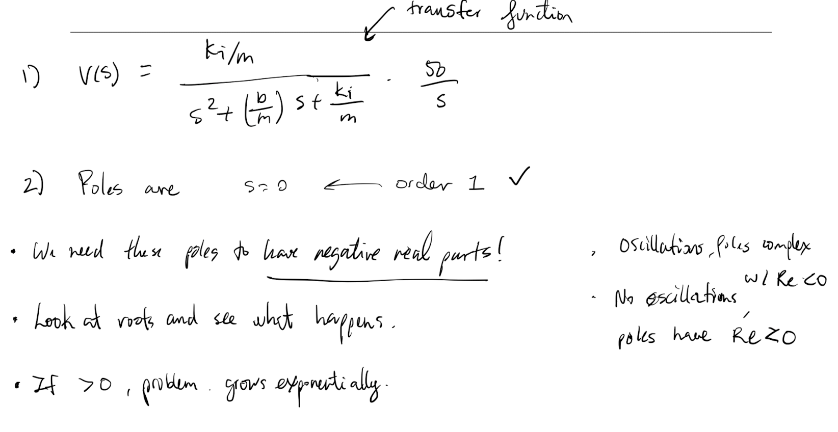
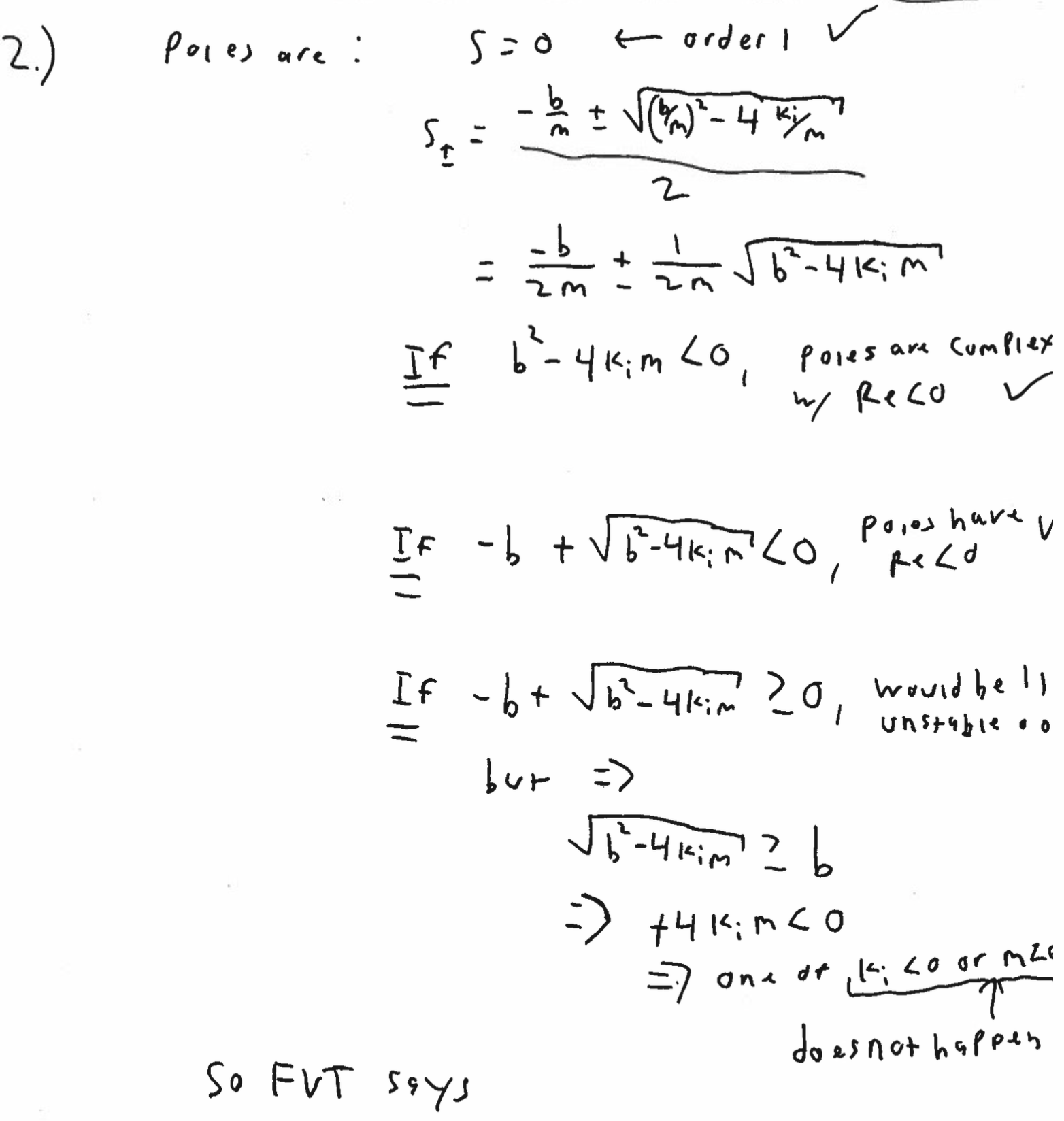
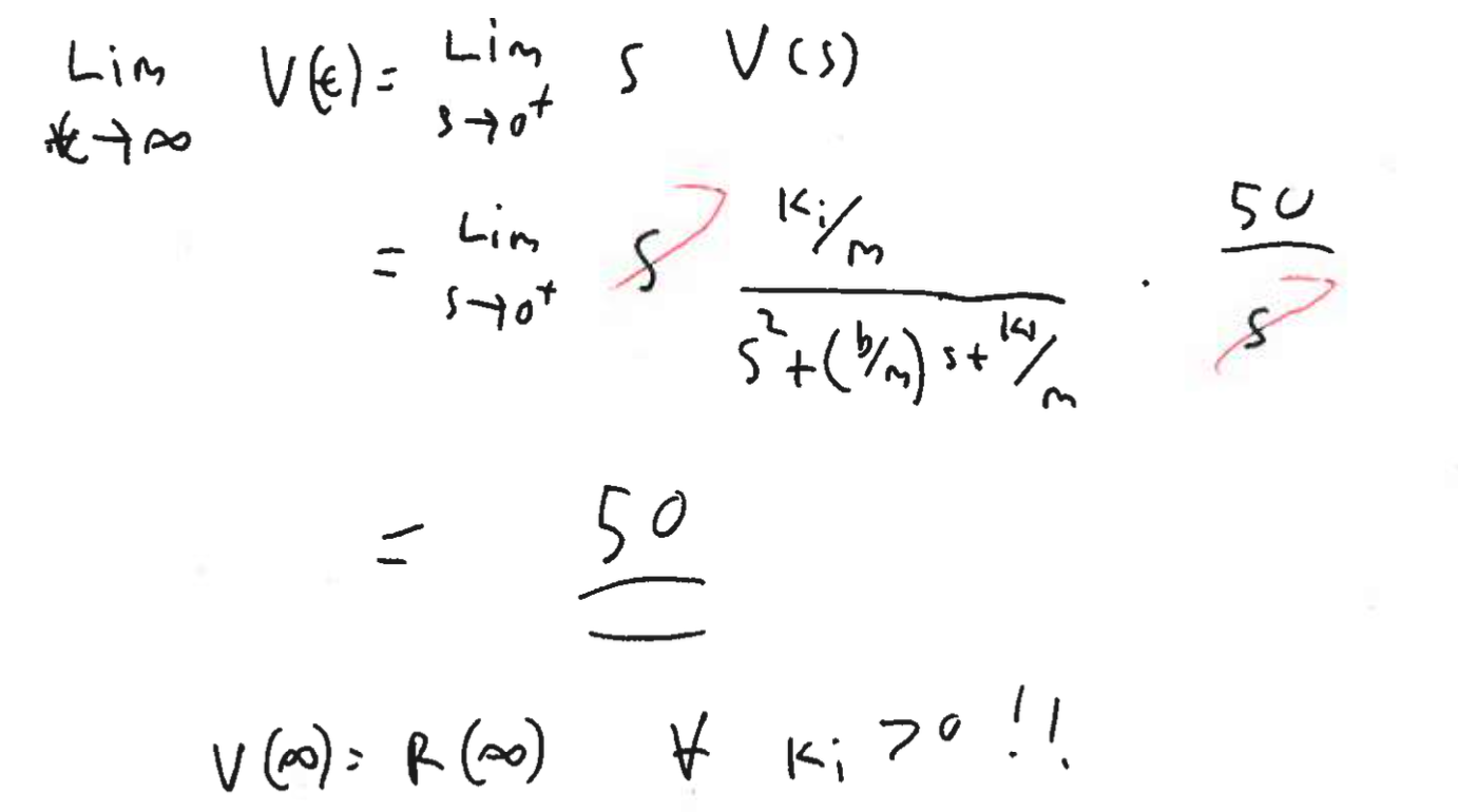
Theorem 3: Final Value Theorem

For a function $F(s)$, if

• is a proper rational function
• has the property that all the poles have real parts that are strictly negative with the exception of a single pole (of order 1)${}^a$ at $s=0$

or if $F(s)$ is the product of a function satisfying the above conditions multiplied by a complex exponential $e^{sT}$, then

${\lim }_{t\to \infty }f(t)={\lim }_{s\to 0}sF(s)$.

If the poles of a rational function do not satisfy the above condition, then ${\lim }_{t\to \infty }f(t)$ does not exist.

${}^a$i.e. $\frac{A}{s}$

Understanding this theorem:

• When it applies, the above gives us a way of computing the “final value” of $f(t)$ from $F(s)$ without computing the inverse Laplace transform and instead evaluating a limit in the complex plane.
• Again $s$ is generally complex so the limit is in the complex plane NOT the real number line. Limits at finite points in the complex plane are a bit different from infinite limits.
  • Here the formal definition of a limit of a complex valued function $F(z)$ at $x_{0\in }\mathbb{C}$ is the constant $L\in \mathbb{C}$ such that for every $ϵ\in {\mathbb{R}}^{+}$ there is a $\delta \in {\mathbb{R}}^{+}$ such that if $|z-z_0|<\delta$ then $|F(z)-L|<ϵ$ where $|\cdot |$ is the standard modulus function.
  • In practice for any problems of computing limits at 0, you can treat the limit as the standard limit you are used to working with.
• Connection to 2D limits from MATH119 - Calculus 2 for Enginering.
  • Provided that the limits exist, we have

$$\underset{s\to 0}{\lim }F(s)=\underset{(a,b)\to (0,0)}{\lim }Re(F(a+bj))+j\underset{(a,b)\to (0,0)}{\lim }Im(F)a+bj$$

Examples in notes.

Note

When the final value theorem does not apply, we do not know if the limit diverges or if it oscillates. Hence, we need more math to be able to ascertain if a solution is bounded or not (without computing the inverse transform)! See examples 8C and 8E for unstable systems and D for a stable but non-convergent system.

Lecture 8 - Zero-input, zero state response, and the delta function

Lecture goals:

• understand how poles effect the inverse Laplace transform
• what the zero-input and zero-state are
• know what the delta function is and its properties are

Understand Poles:

The final value theorem is useful but we can actually do a bit better so we will examine and analyze all the various cases of a function with a single pole. Consider a function $F(s)$ with a single pole of (natural number greater than 1) order $n$ at $a+bi$:

$$f(t)=\frac{1}{(s-(a+bi){)}^n}$$

Taking the inverse Laplace transform gives:

Thus all functions that have a rational Laplace transform (the ones we have covered thus far), have an inverse transform of the form of a weighted sum of terms of the form of the above.

We hence analyze these functions via case analysis!

In conclusion the location of the poles tells us about the behaviour of the solution at infinity (via the final value theorem) but also the initial values (via the initial value theorem).

If only… there was a way to control where the poles are and to thus control the behaviour of the solution to a DE we care about…

Enter the ideas of the zero-input response, the zero-state responses and the transfer function

Definition 1: Zero-State and Zero-Input Response and the Transfer function

Given a linear DE with constant coefficients of the form

$\frac{d^n}{d{t}^n}y+a_{n-1}\frac{d^{n-1}}{d{t}^{n-1}}+...+a_{0}y=f(t)$

along with the needed initial conditions $y(0),y^{\prime }(0),...,y^{(n-1)}(0)$, the Laplace transform of the equation will be of the form

$Y(s)=\frac{F(s)}{s^n+a_{n-1}{s}^{n-1}+...+a_0}+\frac{g(a_0,...,a_{n-1},y(0),...,y^{(n-1)}(0))}{s^n+a_{n-1}{s}^{n-1}+...+a_0}$

where $g$ is some function of the ICs and coefficients.

• The zero-input response is $\frac{g(a_0,...,a_{n-1},y(0),...,y^{(n-1)}(0))}{s^n+a_{n-1}{s}^{n-1}+...+a_0}$. This is the response of the system of the DE models to the initial conditions (i.e. when the forcing term is 0)
• The zero-state response is $\frac{F(s)}{s^n+a_{n-1}{s}^{n-1}+...+a_0}$. This is the response of the system the DE models to the forcing term (i.e. when the ICs are all 0).
• The transfer function is $\frac{1}{s^n+a_{n-1}{s}^{n-1}+...+a_0}$. This function determines the zero-input and the effect of the forcing term.

To help understand the role of the transfer function in the relation between the zero-input response and the zero-state response, we introduce the idea of generalized functions.

In 1927, Physicist Paul Dirac in his “The physical interpretation link of the quantum dynamics” paper introduced the function now known as the “Dirac delta” function.

Definition 2: Dirac Delta Function

The $\delta (x)$ function is defined as the “function” (called a special function or a distribution) that satisfies the properties that:

$\delta (x)=0$ when $x\ne 0$ ${\int }_{-\infty }^{\infty }\delta (x)=1$

Of course there is no classical function that satisfies the above conditions but we can think of $\delta$ as the limit of a collection of functions which we now explore.

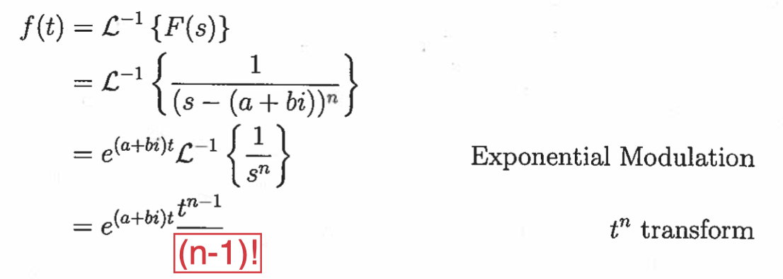
Suppose you hit a nail with a hammer and do a total amount of work of 1 unit. If $f(t)$ is the amount of force applied over time then $1={\int }_0^{t_f}f(t)dt$.

We call this function $\delta (x)$. Mathematically one can make this definition formal but to do so requires a lot of mathematical background.

Theorem 1

If $f$ is a “well-behaved” function defined at $t$ then

${\int }_{-\infty }^{\infty }f(\tau )\delta (t-\tau )d\tau ={\int }_{-\infty }^{\infty }f(t)\delta (t-\tau )d\tau =f(t){\int }_{-\infty }^{\infty }\delta (t-\tau )d\tau =f(t)$.

The above is the main property of the delta function we need.

Example 3:

Transfer function

The transfer function is the systems transform of the impulse function.

In general if $Y(s)=\frac{F_{ap}(s)}{P(s)}$ where $F_{ap}(s)$ is the transform of the forcing term and $P(s)$ is the characteristic polynomial, then

$$y(t)={\mathcal{L}}^{-1}\{\frac{F_{ap}(s)}{P(s)}\}$$ $$=f_{ap}(t)\ast \mathcal{L}\{\frac{1}{P(s)}\}$$ $$=f_{ap}(t)\ast \mathcal{L}\{T(s)\}$$

where $T(s)$ is the system’s transfer function.

Hence a system’s response to any function $f_{ap}(t)$ is simply the convolution of $f_{ap}(t)$ with the systems response to the delta function - called the system’s impulse response.

This is a theorem!

Theorem 2

The zero-state response of a linear DE is the convolution of the input (i.e. forcing term) with the systems impulse response.

With the above results in mind, the solution to any linear DE with constant coefficients can be written as

$$y(t)={\mathcal{L}}^{-1}\{\frac{F(s)}{s^n+a_{n-1}{s}^{n-1}+...+a_0}+\frac{g(a_0,...,a_{n-1},y(0),...,y^{(n-1)}(0),s)}{s^n+a_{n-1}{s}^{n-1}+...+a_0}\}$$ $$=f(t)\ast T(t)+\sum _{k=1}^M{c}_k{t}^{N_k-1}{e}^{{\lambda }_{k}t}$$

where $T$ is the inverse Laplace transform of the transfer function, ${\lambda }_k$ are the poles of the zero-input function, $N_k$ is the order of the $k$th pole, $c_k$ is the coefficient given by the partial fraction decomposition and $M$ is the number of poles (which will always be finite because of the form of the second term).

Lecture 9 - Delta function derivatives and intro to systems and signals

Lecture goals:

• understand how to differentiate the delta function
• know what systems and signals are

Derivatives of $\delta (t)$

It turns out that it is useful to take the derivatives of $\delta (t)$.

In MATH 119 we told you that we can’t differentiate functions at discontinuities so?

Recall that $\delta (t)$ is not a function in the classic sense but is instead a distribution, a collection of functions that have a common property when we take a limit. Hence to differentiate such functions, we need to redefine what it is to be differentiable.

We will not do this formally but will instead play with delta until we magically arrive at the result.

We will start with the derivative of a simpler function.

Examples 1, 2, 3 and 4. Look at notes for solutions.

\delta(t)

Recall it is not a function, but instead a distribution, a collection of functions that have a common property when we take a limit.

Notation 1

${\delta }^{\prime }[f]$ denotes ${\int }_{-\infty }^{t}f(t){\delta }^{\prime }(t)dt$ which is the effect of ${\delta }^{\prime }$ on the test function $f$.

Systems and Signals:

Given a linear differential equations and some specified initial conditions:

$$\frac{d^n}{d{t}^n}y(t)+a_{n-1}(t)\frac{d^{n-1}}{d{t}^{n-1}}y(t)+...+a_0(t)y(t)=f(t)$$ $$y(0)=b_0,...,y^{(n-1)}(0)=b_{n-1}$$

There are two classic problems one considers in engineering.

Definition 1: Analysis and Synthesis

• Analysis: Given a forcing term $f(t)$ solve for $y(t)$.
• Synthesis: Given a $y(t)$, or some conditions on $y(t)$, find a forcing term $f(t)$ such that $y(t)$ solved the differential equation.

We have thus far focused on the analysis problem, which is the easier of the two, but the synthesis problem is generally more useful in engineering design.

To solve the synthesis problem we need a good understanding of how $f(t)$ relates to $y(t)$. Think about the spring problem from L8 Ex2 as an example.

Definition 2: Signals

A signal is a complex-valued function of an independent real variable $t$.

• $t$ usually (but not always) represents time.
• If the domain of the function is $\mathbb{R}$ or some interval of ${\mathbb{R}}^a$ then the signal is said to be a continuous-time (CT) signal.
• If the domain of the function is $\mathbb{Z}$, $\mathbb{Q}$ or other discrete subset of ${\mathbb{R}}^b$ then the signal is said to be a discrete-time (DT) signal.

Definition 3: Systems

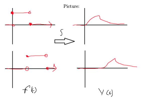
Mathematically, a system is a map from a space of input signals to a space of output signals.

Notation 2

If $S$ represents some system then $f\to y$ or $y(t)=(Sf)(t)$ or simply $y=Sf$ indicated that $y(t)$ is the response (solution) of the system $S$ to the input signal $f(t)$.

The above is similar to systems of equations from 115 and the connection to ma- trices and the “input” and “output” vectors.

Explicitly, the system of equations

$$s_{11}{f}_1+..+s_{1n}{f}_n=y_1$$ $$s_{m1}{f}_1+..+smn{f}_n=y_m$$

can be written as

$$S\overrightarrow{f_1}=\vec{y}$$

Here one can ask the analysis question of solving for $\vec{y}$(“easy”) or the synthesis question of solving for $\vec{f}$(hard”) and generally wants to know the relation between the response and input.

Further, the matrix S is the map between the vector space of input functions (all valid $\vec{f}s$) and the vector space of output functions (all valid $\vec{y}s$).

Definition 4

A system $S$ is continuous-time (CT) if both its input and output signals are CT.

A system $S$ is discrete-time (FT) if both its input and output signals are DT. $S$ is a hybrid system if ti contains both CT and DT signals.

Lecture 10 - Systems and signals introduction continued

Lecture goals:

• know what systems and signals are
• understand the various properties we generally care about

Connection between CT systems and DEs:

A DE represents a CT system only when for any signal in the set of input signals of the system, there is a signal in the output class that satisfied the DE.

Example 1:

Connection between DT systems and difference equations:

DT systems are represented by difference equations. An example of a difference equation is the mine craft chicken model from assignment 1.

Here is another classic fun difference equation

$$x_{n+1}=r{x}_n(1-x_n),r>0$$

This models the normalized population of bunnies with the constraints that

• there is growth proportional to the population for small populations and
• if the population is close to the environmental limit, $1$ in this model, then the population declines.

To Lecture10 magic.m!!

The previous two examples demonstrate that generally speaking we can explore the relation of the input and outputs for many systems by “simply” solving DEs, difference equations etc.

We now examine some more important properties of systems.

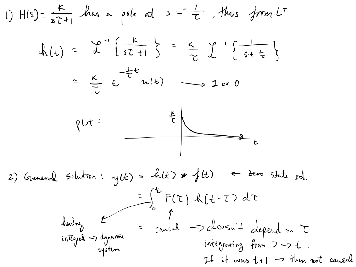
Definition 1: Memoryless vs Dynamic systems

A system is memoryless, if the instantaneous output value $y(t)$ depends only on the input value $f(t)$ at time $t$.

A system that is not memoryless is dynamic.

Most interesting problems involve systems that are dynamic.

Definition 2: Causality

A system $A$ is causal if $y(t)=(Sf)(t)$ only depends on $f(\tau )$ for $\tau \le t$.

Idea: the output signal $y$ only depends on the previous behaviour of $f(t)$ (i.e. not the future values of $f(t)$).

Definition 3: Causality (Alternate Definition)

A system $A$ is causal if for all $t\ge 0$ whenever $f_1(\tau )=f_2(\tau )$ for all $\tau \le t$ and $y_1(t)=(S{f}_1)(t)$ and $y_2(t)=(S{f}_2)(t)$ then $y_1(\tau )=y_2(\tau )$, for all $\tau \le t$.

To see why the last example above is noncausal one needs to notice that $f^{\prime \prime }(t)$ is defined as a limit of a difference quotient and as such it depends on more future information than $y\prime (t)$ does.

Definition 4: Multivariable vs Scalar Systems

A system is multivariable if is has multiple inputs and/or outputs.

A system is scalar if it has a single input and a single output.

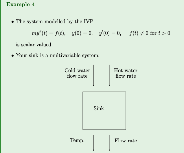
Multivariable systems are harder to control then scalar systems.

We will study scalar systems (but may examine multivariable systems a bit).

Definition 5: Linearity

A system S is linear if it has the property that if $f(t)$ and $g(t)$ are input signals and $\alpha$, $\beta \in \mathbb{C}$ then

$S(\alpha f_1+\beta f_{2)}=\alpha S(f_1)+\beta S(f_2)$

In simpler terms, it means that if you have a system that is linear, then scaling the input signal by a constant ($\alpha$) and adding it to another scaled input signal by another constant ($\beta$) will have the same effect on the output signal as scaling and adding the output signals individually. This property is fundamental in many areas of engineering and mathematics, particularly in signal processing and control theory.

Note if $\theta \ll 1$ then $sin(\theta )\approx \theta$ and we can approximate the full pendulum by the linear oscillator:

$$m{l}^{22{\theta }^{\prime \prime }(t)+mgl\theta }=0,y^{\prime }(0)=y_1$$

Linear systems are “easy” to study but tend to have “simpler dynamics” than non- linear systems.

Definition 6: Time-invariance

A system is time-invariant if its response does not change with time.

Explicitly if $f(t)\to y(t)$ then for all $T\in \mathbb{R},f(t-T)\to y(t-T)$.

A system that is not time-invariant is called time-variant.

Definition 6 defines time-invariance for a system. A system is considered time-invariant if its response remains the same regardless of shifts in time. Mathematically, if an input signal $f(t)$ produces an output signal y(t)y(t), then for any time shift $T$, if the input signal $f(t-T)$ is applied to the system, the output $y(t-T)$ remains the same.

For the rest of this course we will focus on linear time invariant systems of LTSs.

These systems are often modelled by constant-coefficient ODES and hence our work on the Laplace transform can be used to study the system…

Lecture 11 - Midterm Review

Do the examples.

Example 1:

• I don’t understand how to solve example 1. Wow, what a start.
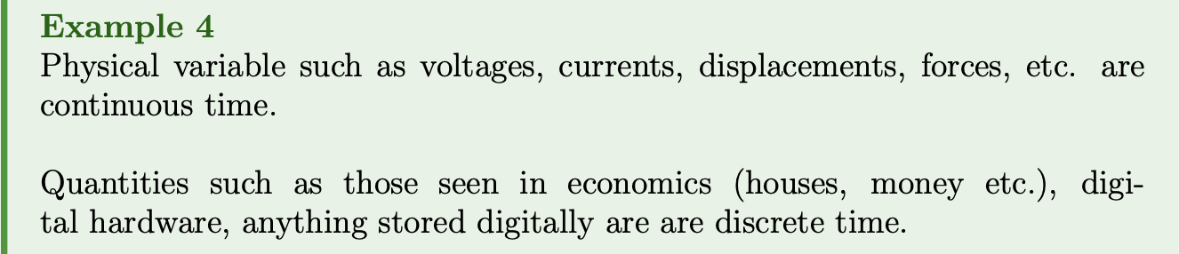
• How do you differentiate between continuous and discrete time??

1. Continuous time vs discrete time: Since the independent variable $t$ is continuous, this system is a continuous-time (CT) system.
2. Memoryless vs dynamic: The presence of terms like $y(t)$, $y^4(t)$, and $y^6(t)$ indicates that the system has dynamic behaviour. Therefore, it is a dynamic system.
3. Causal vs non-causal: In the equation $y^6(t)+y^4(t)+6y(t)=f(t)$, the output $y(t)$ depends on the current and past values of itself ($y(t)$, $y^4(t)$, and $y^6(t)$), which means it only depends on past or present inputs. Therefore, the system is causal.
4. Multivariable vs scalar: This system has a single input ($f(t)$) and a single output ($y(t)$), making it a scalar system.
5. Linear vs nonlinear: The system equation $y^6(t)+y^4(t)+6y(t)=f(t)$ involves nonlinear terms like $y^6(t)$ and $y^4(t)$, so the system is nonlinear.
6. Time-invariant vs time-variant:A system is time-invariant if its response does not change with time. In other words, if we shift the input signal in time, the output signal should shift by the same amount.

For a time-invariant system, shifting the input signal $f(t)$ by $T$ should result in a corresponding shift in the output signal $y(t)$ by $T$.

Let’s examine if this holds true for the given equation:

If we shift $f(t)$ by $T$, we get $f(t-T)$. The corresponding output $y(t-T)$ should satisfy the equation:

y6(t−T)+y4(t−T)+6y(t−T)=f(t−T)y6(t−T)+y4(t−T)+6y(t−T)=f(t−T)

Since the equation remains the same after the time shift, the system is time-invariant.

In summary:

• Continuous time
• Dynamic
• Non-causal
• Scalar
• Nonlinear
• Time-variant

Example 2:

Memorize

$e^{wtj}=cos(wt)+jsin(wt)$ and $e^{-wtj}=cos(wt)-jsin(wt)$

Example 3: (Partial Fraction)

Example 4: Solve IVP

Have the options between PF or Convolution

Example 5: Solve IVP

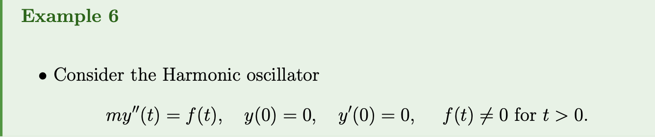
Example 6:

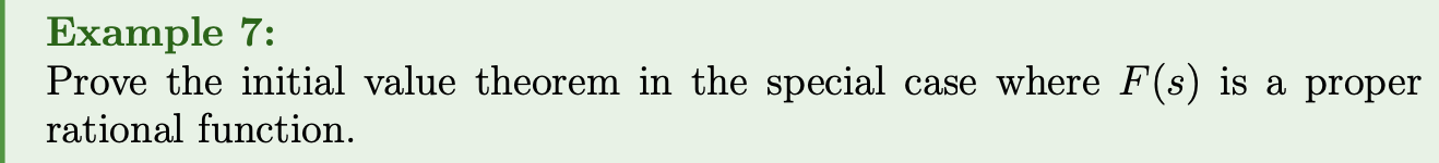
Example 7: Write inverse Laplace transform of…

Lecture 12 - Fun with Foreshadowing (Looking ahead)

In the synthesis problem we are given $y(t)$ and want to find $f(t)$. Later we will cover how to do this in mathematical detail but… how do we in principle do this??? Let’s look at an example!

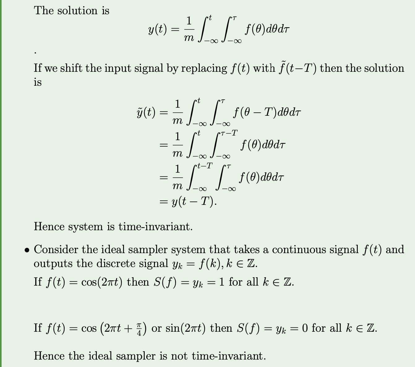
Solution: The solution is

$${y(t)={\int }_0^{t}f(\tau ){\mathcal{L}}^{-1}\{\frac{1}{m{s}^2+\mu s}\}|}_{t-\tau }$$

To compute the inverse Laplace transform note that

$$\frac{1}{m{s}^2+\mu s}=\frac{1}{s(ms+\mu )}$$ $$=\frac{1}{\mu s}-\frac{m}{\mu (ms+\mu )}$$ $$\frac{1}{\mu s}-\frac{1}{\mu (s+\frac{\mu }{m})}$$

Hence, by exponential modulation in the Laplace table

$${\mathcal{L}}^{-1}\{\frac{1}{m{s}^2+\mu s}\}=\frac{1}{\mu }-\frac{1}{\mu }{e}^{-\frac{\mu t}{m}}$$

Combining this with the previous result gives

$$y(t)={\int }_0^{t}f(\tau )(\frac{1}{\mu }-\frac{1}{\mu }{e}^{-\frac{\mu (t-\tau )}{m}})d\tau$$

Now suppose that we want to find $f(t)$ such that $y(t)$ is given by a particular provided function. In the next few examples, we will derive a $P$ controller that is commonly used to solve this problem in real time.

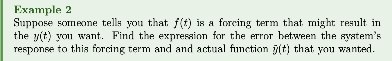
The response of the system to $f(t)$ is given by

$$y(t)={\int }_0^{t}f(\tau )\left(\frac{1}{\mu }-\frac{1}{\mu }{e}^{-\frac{\mu (t-\tau )}{m}}\right)d\tau$$

and hence the error is

$$\tilde{y}(t)-{\int }_0^{t}f(\tau )\left(\frac{1}{\mu }-\frac{1}{\mu }{e}^{-\frac{\mu (t-\tau )}{m}}\right)d\tau$$

If the error is 0 for all values of $t$, then we found the solution to the synthesis problem!

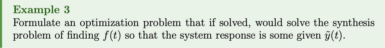
We thus want to pick $f(t)$ (ideally that is smooth) such that the error is as close to 0 as possible. Hence we want to solve the optimization problem

$$min\left|\tilde{y}-{\int }_0^{t}f(\tau )\left(\frac{1}{\mu }-\frac{1}{\mu }{e}^{-\frac{\mu (t-\tau )}{m}}\right)d\tau \right|$$

In the above there are few different ways to define what we mean by min. Two common ones are

• Minimize the maximum value over all $t$ i.e. the $L_{\infty }$ norm
• Minimize the average value i.e. the $L_1$

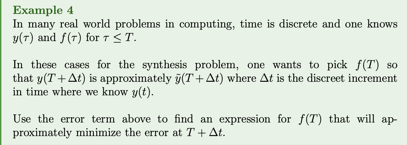
The (signed) error at $T+\Delta t$ is given by

$$E(T+\Delta t)=\tilde{y}(T+\Delta )-{\int }_0^{T+\Delta t}f(\tau )\left(\frac{1}{\mu }-\frac{1}{\mu }{e}^{-\frac{\mu (t-\tau )}{m}}\right)d\tau$$ $$=E(T)+\tilde{y}(T+\Delta )-\tilde{y}(T)-{\int }_T^{T+\Delta }f(\tau )\left(\frac{1}{\mu }-\frac{1}{\mu }{e}^{-\frac{\mu (t-\tau )}{m}}\right)d\tau$$

Assuming $\tilde{y}(t)$ is continuous and $\Delta t$ is small, we can write

$$\tilde{y}(T+\Delta t)-\tilde{y}(T)\approx 0$$

and

$${\int }_T^{T+\Delta t}f(\tau )(\frac{1}{\mu }-\frac{1}{\mu }{e}^{-\frac{\mu (t-\tau )}{m}})d\tau \approx f(T){\int }_T^{T+\Delta t}(\frac{1}{\mu }-\frac{1}{\mu }{e}^{-\frac{\mu (t-\tau )}{m}})d\tau =k_{p}f(T)$$

where $k_p$ is some number (formally it is the integral but we don’t want to compute it in practice…). Thus

$$E(T+\Delta t)\approx E(T)-k_{p}f(T).$$

If we want $E(T+\Delta t)=0$ then we can pick $f(T)\approx \frac{E(T)}{k_p}$ which we will write as $f(T)=k_{p}E(T)$ where $k_p$ is non-zero constant.

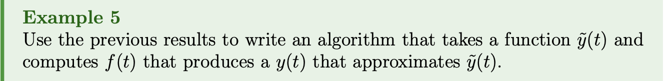
Here is some pseudocode

Define y_want(t), kp, the error at t=a and
the convolution kernal, G, for the given DE.
for t=0:Dt:b
	f(t+Dt) = kp*E(t)
	y(t+Dt) = num_int(f(u)*G(t-u*), u, 0, t+Dt)
	E(t+Dt) = y_want(T+Dt)-y(t+Dt)
end for

In the above num_int is some numerical method that integrates.

Lecture12_basic_PID.m implements a method that uses the above pseudocode with extra controls for the integral and derivative of the error.

Lecture 13 - Systems Input and Responses

Lecture goals:

• understand the impulse response of an LTI
• the convolution properties of LTIs
• response of an LIT to exponential inputs

Recap of some DE results:

Recall that for a linear DE with constant coefficients the zero state response is

$$Y(s)=H(s)F(s)$$

where:

• $Y(s)$ is the Laplace transform of the output signal,
• $H(s)$ is the transfer function of the DE, and
• $F(s)$ is the Laplace transform of the forcing term (input signal).

If the forcing term is the delta impulse function (i.e. $f(t)=\delta (t)$), then $F(s)=1$ and thus

$$Y(s)=H(t)\times 1=H(t)$$

In this case, $H(s)$ represents the response of the system to an impulse input. Consequently, the inverse Laplace transform of $H(s)$, denoted as $h(t)={\mathcal{L}}^{-1}\{H(s)\}$, is termed the impulse response of the DE. The impulse response describes the behaviour of the system when subjected to an impulse input, which is often a critical characteristic in analyzing system dynamics and properties.

Thus we also call

$$h(t)={\mathcal{L}}^{-1}\{H(s)\}$$

the impulse response of the DE.

Understanding the impulse response of an LTI system is fundamental, as it provides insights into how the system responds to sudden changes or impulses in the input signal.

Note

That this is simply the zero-state response to a unit impulse. Thus when we write

$Y(s)=H(s)F(s)$

the transfer function, $H(s)$, is always just the Laplace transform of the impulse response.

Finally by the convolution theorem the zero-state solution is simply

$$y(t)=(h\ast f)(t).$$

More explanation

Furthermore, by the convolution theorem, the zero-state solution (the solution without considering initial conditions) can be expressed as the convolution of the impulse response $h(t)$ with the input signal $f(t)$, denoted as $(h\ast f)(t)$.

In summary, the transfer function encapsulates the system’s behaviour and characteristics, particularly its response to an impulse input. The convolution theorem provides a powerful tool for analyzing LTI systems by relating the input and output signals through convolution with the impulse response. Understanding these concepts is crucial for analyzing and designing LTI systems in various engineering applications.

$h(t)$ is the impulse?

Impulse response of a LTI:

The above holds for Linear DEs with constant coefficients but what about more general LTIs. In general theses might not be able to be modelled by a DE… so how do we find their responses to general inputs.

Theorem 1

The response of an LTI system is the convolution of the input with the system’s impulse response.

Proving this in the CT case is a bit messy so we will show that the result holds for the DT case and then make the connection to the CT case.

First we need to define some DT analogues of CT objects we have worked with.

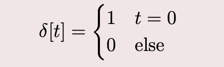
Definition 1: Kronecker delta

The Kronecker delta function $\delta [t]$ is defined as the function from $\mathbb{Z}$ to $\{0,1\}$ given by:

Theorem 2

For all functions $f:\mathbb{Z}\to \mathbb{C}$ $f[t]=\sum _{\tau =-\infty }^{\infty }f[\tau ]\delta [\tau -t]$

Theorem 2 shows how to decompose every function $f$ into a linear combination of impulse functions (i.e. $\{\delta [\tau -t]|\tau \in \mathbb{Z}\}$ is a basis for all DT functions.)

Proof of Theorem 1: in notes.

Clarifications on Theorem 3 and 4

Theorems 3 and 4 provide further insights into the behavior of Linear Time-Invariant (LTI) systems, particularly regarding their response to different types of inputs and how this behavior can be analyzed using the Laplace transform.

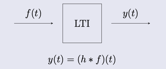
Theorem 3: More explicit version of Theorem 1

Given the LTI

where $h(t)$ is the impulse response of the system.

Theorem 4: LTI response to an exponential

If $S:f\to y$ is a LTI then for any $s\in \mathbb{C}$ $e^{st}\to H(s)e^{st}$ where $H(s)$ is the LT of the system’s impulse response and is called system’s transfer function.

Note this means that complex exponentials are the eigenfunctions of LTIs and the transfer function tells you the eigenvalues of the system! (like with DEs)

Thm 4 explanation

This theorem states that if $S:f\to y$ represents an LTI system, then the response of the system to a complex exponential input $e^{st}$ is given by $H(s)e^{st}$, where $H(s)$ is the Laplace transform of the system’s impulse response. This $H(s)$ is referred to as the system’s transfer function. Furthermore, it highlights that complex exponentials are eigenfunctions of LTI systems, and the transfer function provides information about the eigenvalues (poles) of the system, similar to the behaviour of differential equations.

Proof: in notes.

TLDR; In general the response of a LTI system to an input f(t) is given by

$$y(t)=(h\ast f)(t)$$

and since the eigenfunctions of LTIs are complex exponentials, we can decompose $f(t)$ into eigenbasis of complex exponentials (like we did with DEs).

In the frequency domain we have

$$Y(s)=H(s)F(s)$$

Hence, if we want to analyze the system we can replace convolution with multiplication and simply analyze the system based on its eigenfunction decomposition, poles, etc. (like we did with DEs).

Lecture 14 - Transfer functions, Responses and the standard first order system

Lecture goals

• Understand the connection between our previous material for DEs and systems
• Know what the standard 1st order system is

If a system is able to be modelled by a linear DE with constant coefficients, i.e. $D(y(t))=f(t)$, then the transfer function can be obtained from the differential equation.

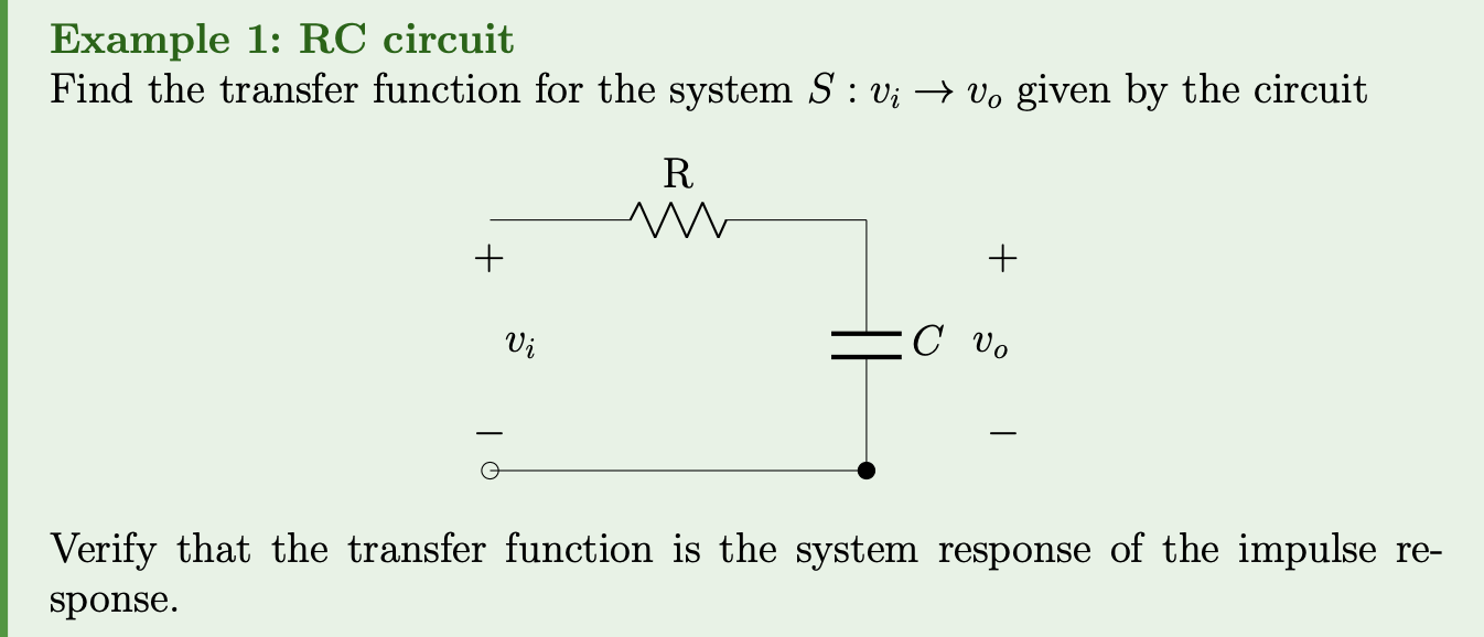
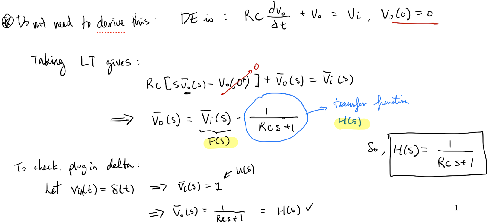
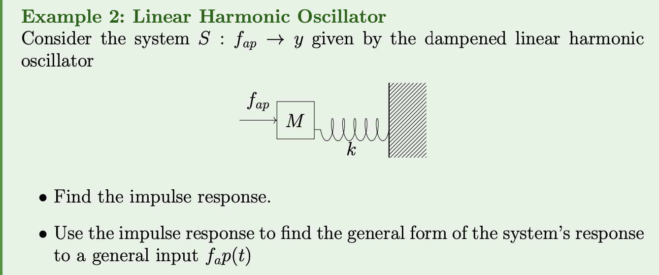
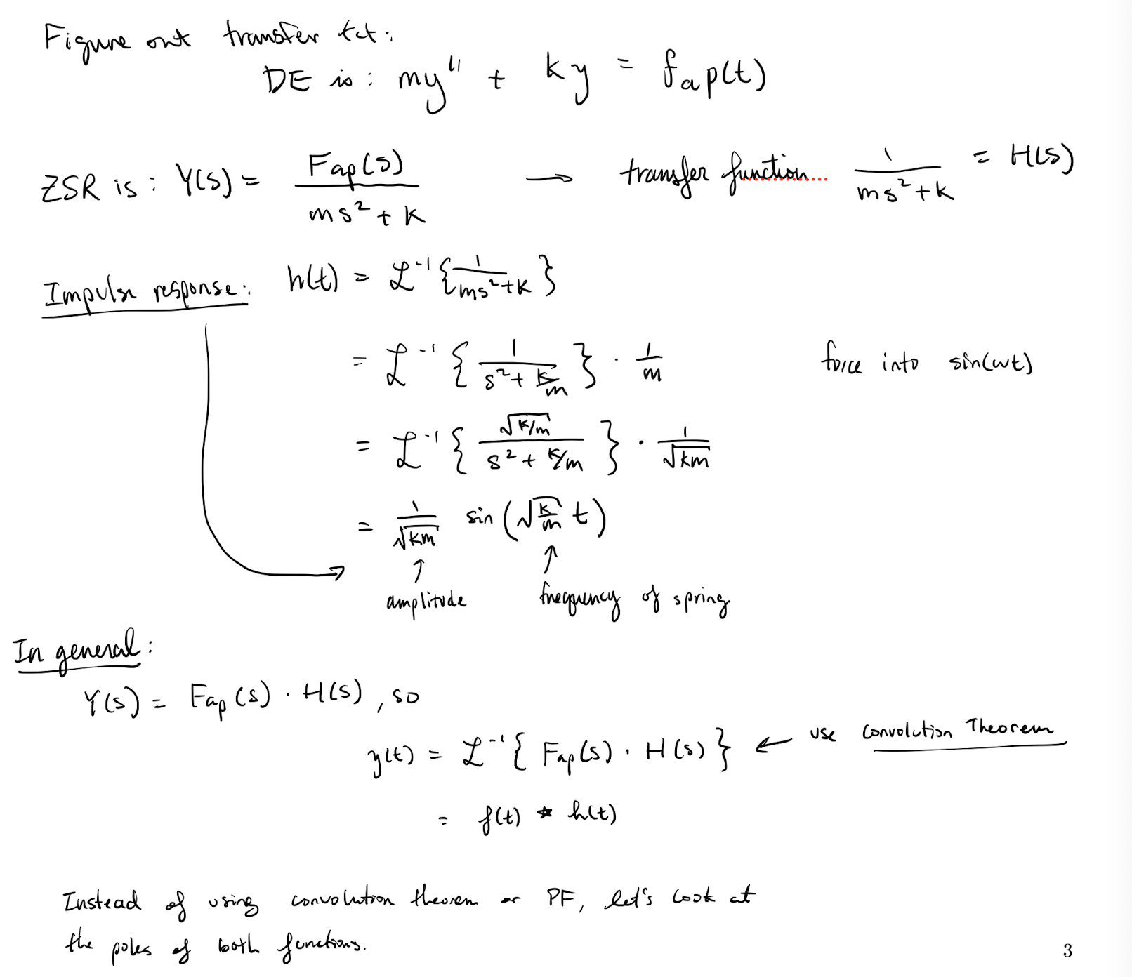
These examples

These examples illustrate the application of transfer functions and impulse responses in analyzing system behavior. The first example involves an RC circuit, a common electrical system, while the second example deals with a dampened linear harmonic oscillator, a common mechanical system.

Understanding these examples helps in grasping the practical applications of transfer functions and responses in various engineering systems. It also highlights the connection between differential equations and system analysis, showing how concepts from one domain can be applied to understand and analyze systems in another domain.

A few things to note:

• In general $F_{a}p(s)$ can have poles of its own and thus the system response to will reflect the poles of both the transfer function, $H(s)$, and the LT of the forcing term $f_{a}p(t)$.
• The effects of the transfer function are present for any input so it is particularly important to understand the effects of the poles (and zeros) of $H(s)$.
• We will mostly look at the cases where the input is a unit impulse, $\delta (t)$, or a unit step, $u(t)$. Recall from A3 Q3 that for a second order DE these terms allow us to effectively set the initial condition at $0^{+}$ for the system.
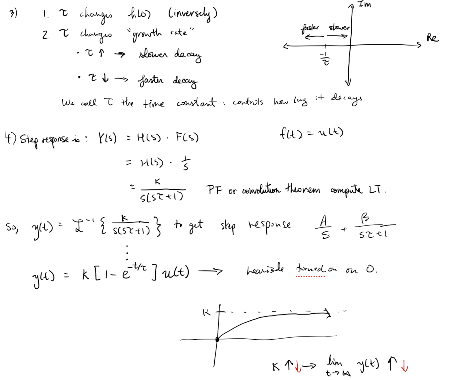
  • The response to the unit step impulse is $Y(s)=H(s)$.
  • The response to the unit step impulse is $Y(s)=\frac{1}{s}H(s)$.
  • The step response is the integral of the impulse response (subtle connection to L12…)

In the “real world” it is often easier to physically generate a unit step function than a unity impulse so point 2 above gives us a nice way to compute transfer functions.

Understanding general system responses

Recall that all polynomials with real valued coefficients can be factored into a product of linear and quadratic terms. Hence if we want to understand the system response of any system, it is sufficient to understand how first and second order linear systems respond. We will thus explore the standard 1st and 2nd order systems in detail. All other LITs can be studied by taking a linear combination of the results of the standard systems.

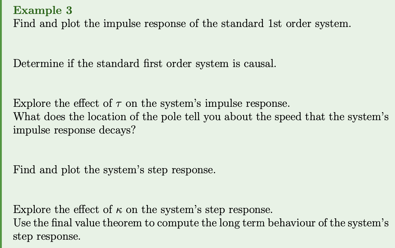
Definition 1: Standard 1st order system

The standard 1st order system has the transfer function $H(s)=\frac{\kappa }{s\tau +1}$ where $\kappa ,\tau >0$. $\kappa$ is called the DC gain and $\tau$ is called the time constant.

In this transfer function:

• $\kappa$ represents the gain of the system at DC (zero frequency).
• $\tau$ determines the rate at which the system responds to input changes. A larger ττ indicates slower response, while a smaller ττ indicates faster response.

Lecture 15 - Basic Control Theory - Cruise Control

Lecture goals:

• Understand the basic of closed control loops
• What proportional and integral control systems are
• Their benefits/limitations and how to set them up to control a system

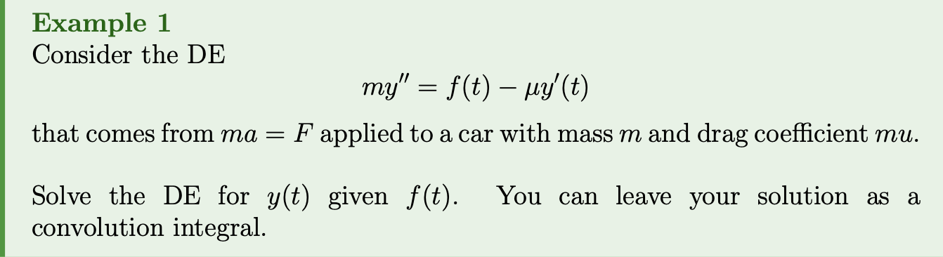
Consider the simple system that models the velocity of a vehicle:

$$m{v}^{\prime }(t)+bv(t)=f(t)$$

where $v(t)$ is the velocity of the vehicle, $m$ is the mass, $b$ is the coefficient of drag and $f(t)$ is the velocity forcing term which is a combination of the effects of the engine/brakes as well as the effects of the road (hills etc).

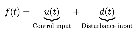
It is nice to split up the input into terms we can control (brakes/gas) and terms we can’t (road conditions):

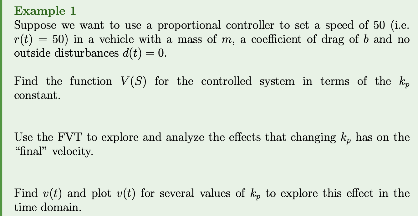
Goal: Find $u(t)$ so that the vehicle velocity $v(t)$ follows some given reference input, $r(t)$.

Solution: We use a “controller” to adjust $u(t)$ to obtain our desired velocity. We do this is frequency space.

We examine two options.

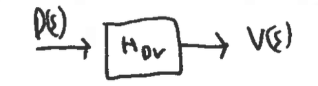
Open loop controller:

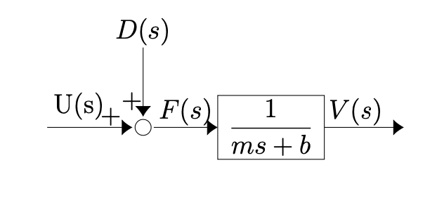
The box is the car system $H(s)$.

Here:

• $U(s)$ is the Laplace transform of the control input.
• $D(s)$ is the Laplace transform of the disturbance input.
• $F(s)$ is the Laplace transform of the total forcing term. ($F(s)=U(s)+D(s)$)
• $V(s)$ is the Laplace transform of the resulting velocity.

These controllers only work well if we know the disturbance the system undergoes, if the system always needs a constant known output or if the user can make adjustments as needed.

Some applications include washer/dryers for clothing, toasters, watering systems, step motors etc but open loop systems do not work well for our application.

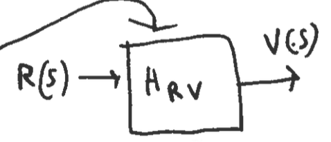
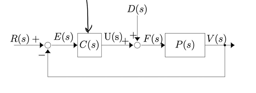
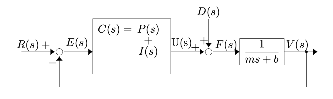
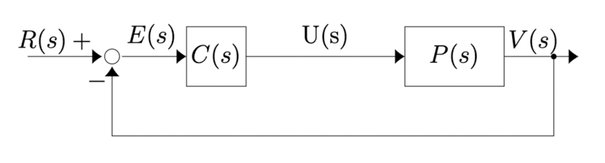
Closed loop controller:

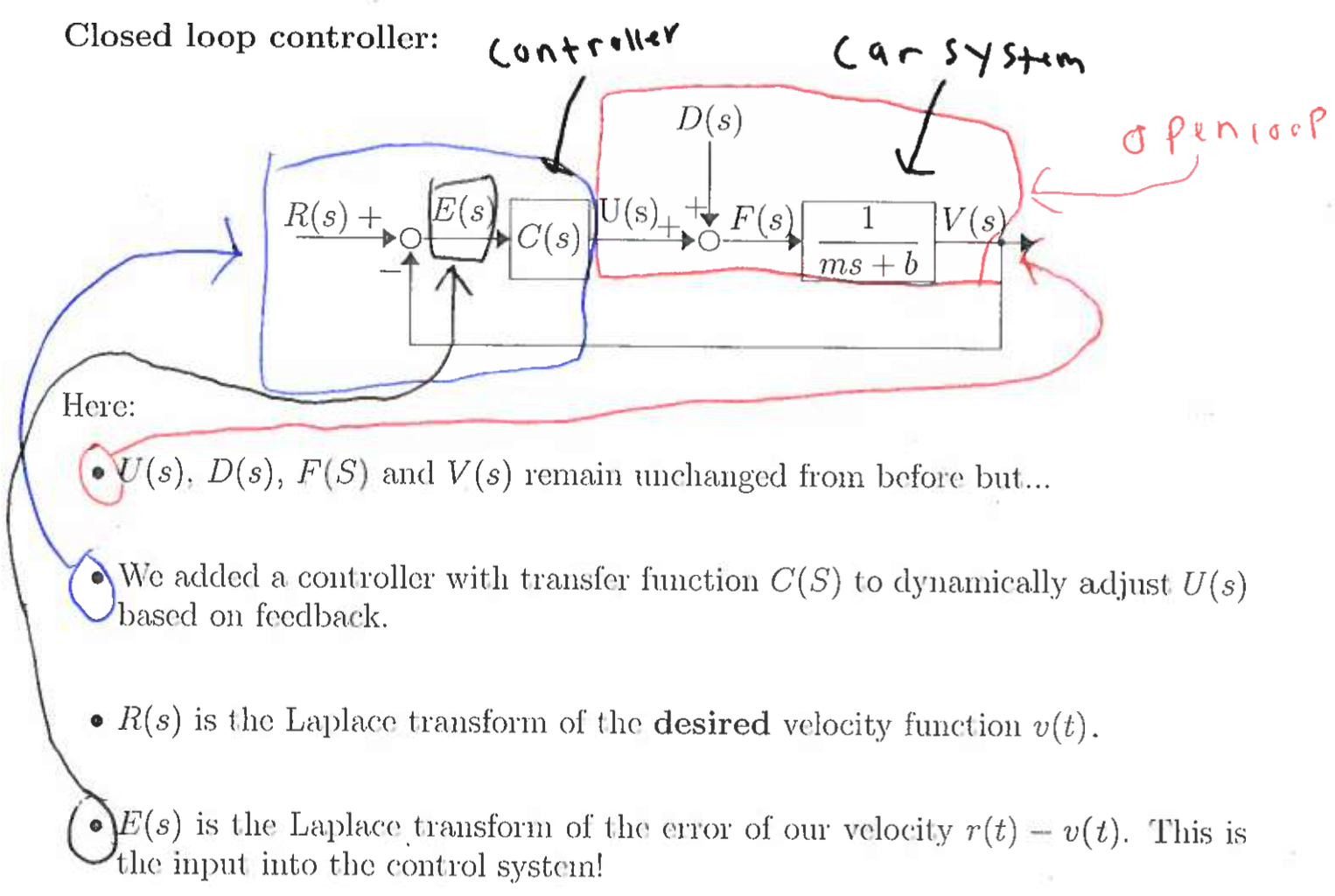
Here:

• $U(s),D(s),F(s)$ and $V(s)$ remain unchanged from before but…
• We added a controller with transfer function $C(s)$ to dynamically adjust $U(s)$ based on feedback.
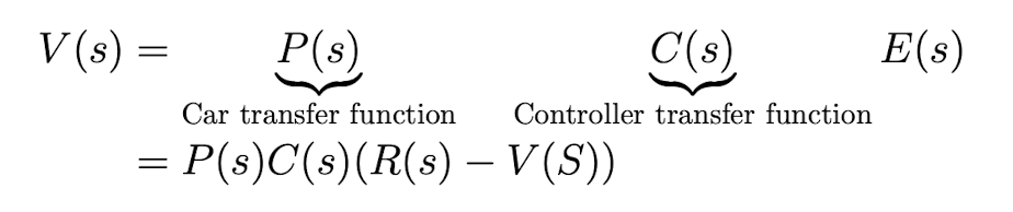
• $R(s)$ is the Laplace transform of the desired velocity function $v(t)$.
• $E(s)$ is the Laplace transform of the error of our velocity $r(t)-v(t)$. This is the input into the control system!

New Goal: Find a transfer function $C(s)$ such that $E(s)=0$ (as $t\to \infty$) and hence we have the desired velocity i.e. $V(s)=R(s)$.

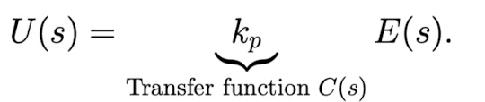
Proportional control:

Idea: Let $u(t)=k_{p}e(t)$ for $k_p\in {\mathbb{R}}_{>0}$. In this case

• if $e(t)>0$ then we “hit the gas” to speed up,
• if $e(t)<0$ we “hit the breaks” to slow down and
• if $e(t)=0$ we do nothing.

We will explore how this works in the case where $D(s)=0$.

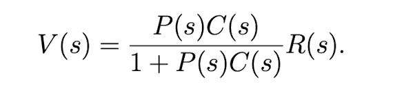
If we use this controller then

We have

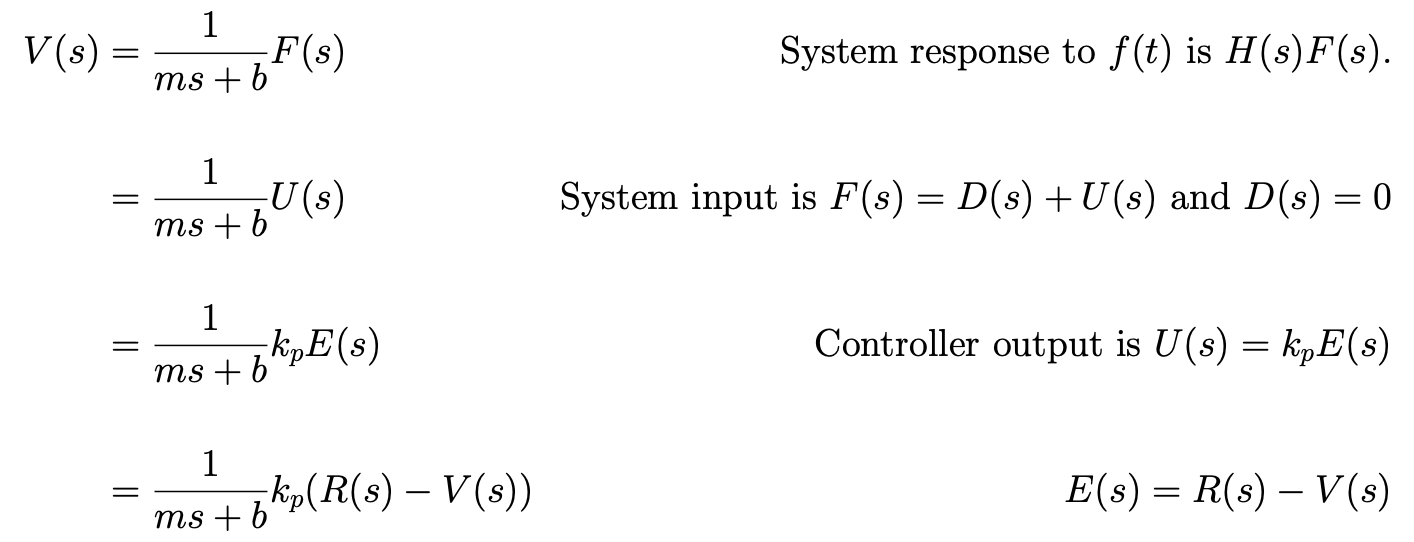
Solve for $V(s)$:

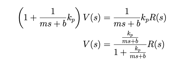
Let’s write this in standard form:

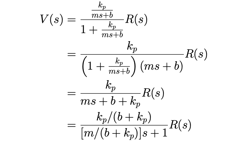
Just algebra. $V(s)$: What comes out of the system (the fraction) given $R(s)$.

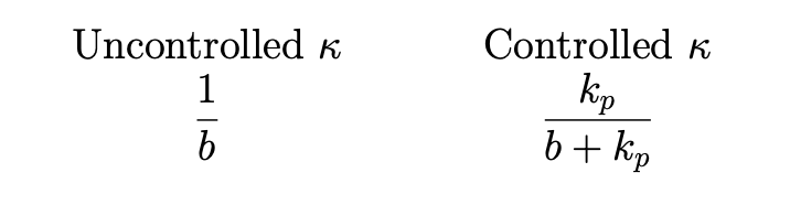
The transfer function for the controlled system is

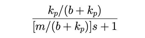
which is the transfer function for a first order system with a DC gain of (number on top. Defined in the last lecture.)

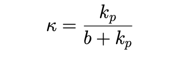
and a time constant of

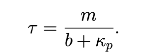
This transfer function looks similar to the transfer function for the uncontrolled car:

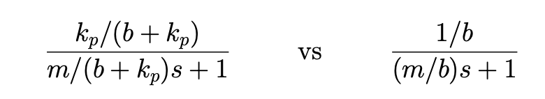
but we can now adjust the DC gain and time constants by changing $k_p$.

We will call this transfer function for the controlled system

Controlled system

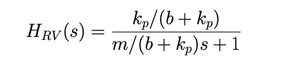
$RV$ because it controls based on $R$ and $V$.

If we want to account for a disturbance term, we can simply find a transfer function $H_{DV}(s)$ such that $V(s)=H_{DV}(s)D(s)$.

Pic:

By linear superposition (all the systems are linear) the net response would be

$$V(s)=H_{RV}(s)R(s)+D_{DV}(s)D(s)$$

Note

We usually just consider $R(s)=0$ for this course.

Now, we want to pick $k_p$ appropriately so that the system does what we want.

Changing $k_p$ lets us

• Adjust the time constant:

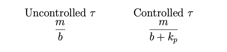
For larger values of $k_p$, $\tau$ becomes smaller.

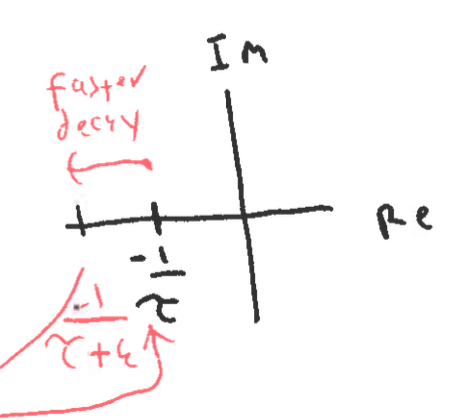
Recall that a smaller $\tau$ leads to a faster decay to the “final” value of the system (which always exists for the standard first order system).

• Adjust the DC gain

by changing $k_p$, we can make $\kappa$ obtain any value between 0 and 1.

Insert the answers…todo

To see the effects of $k_p$ in the time domain run Lecture15_pcontroller.m.

Major limitation: If $e(t)$ is ever 0 then $u(t)=k_{p}r(t)=0$.

Thus in the absence of any disturbance to the system (i.e. $d(t)=0$), the input into the system $f(t)$ also vanishes.

Thus, there is no system input and hence $v(t)$ will drop (since $b>0$).

In general $p$ controllers can never achieve the perfect asymptotic velocity!

While in this example, we can get as close to the desired velocity as we want, in for higher order systems $p$ controllers tend to overshoot and potentially become unstable for large values of $k_p$.

Hence we introduce

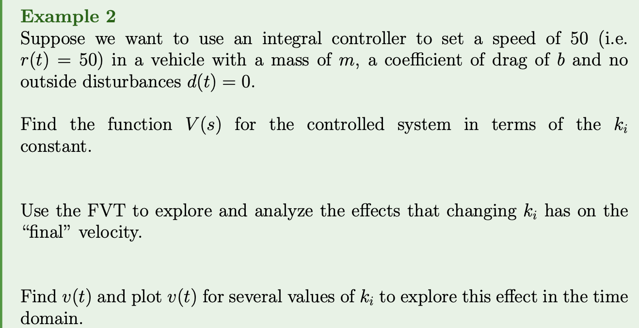
Integral controllers: (average the error!)

Let the error term be proportional to the integral of the error:

$$c(t)=k_i{\int }_0^{t}e(\tau )d\tau$$

This will go to zero exactly when the average error is 0. (This controls the average.)

Pic:

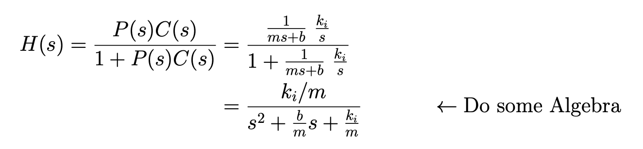
It can hence (in principle) bring the average error to 0! We hence repeat the same analysis to this new controller. (What changed? Nothing except $C(s)$)

The transfer function for the integral term is $U(s)=\frac{k_i}{s}$ (Hw 4 Q1).todo

Hence

so

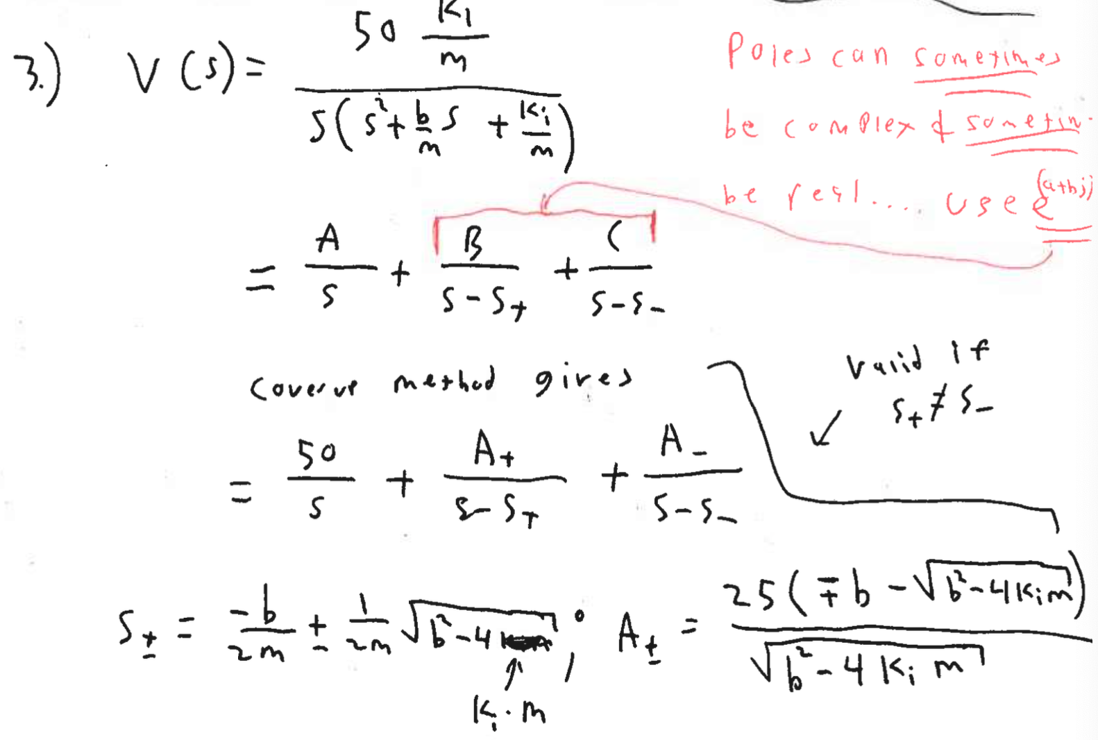
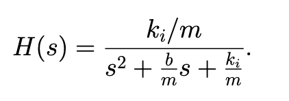
Thus the new controlled system has a transfer function of

How is this different from the first one?

This one is squared!! Notice $s^2$.

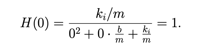
This is the transfer function for a second order system ($s^2$) so we will delay its full analysis until we cover the standard second order system in the next lecture but the DC gain is

Now let’s play with this system a bit more.

To see the effects of $k_p$ in the time domain run Lecture15pcontroller.m Major Limitations:

• Since we adjust based on the integral the error, integral controllers do strongly quickly adjust to changes. i.e. they “adjust the average”
• The above leads to the potential to overshooting the goal velocity. This is also in part because the solutions generally with come in conjugate pairs and hence the solution will have sinusoidal terms that will decay to 0.

Lecture 16 - Standard 2nd order system, PI controllers and extra poles

Lecture goals:

• Understand the basics of the standard second order system
• Know what a PI controller is.

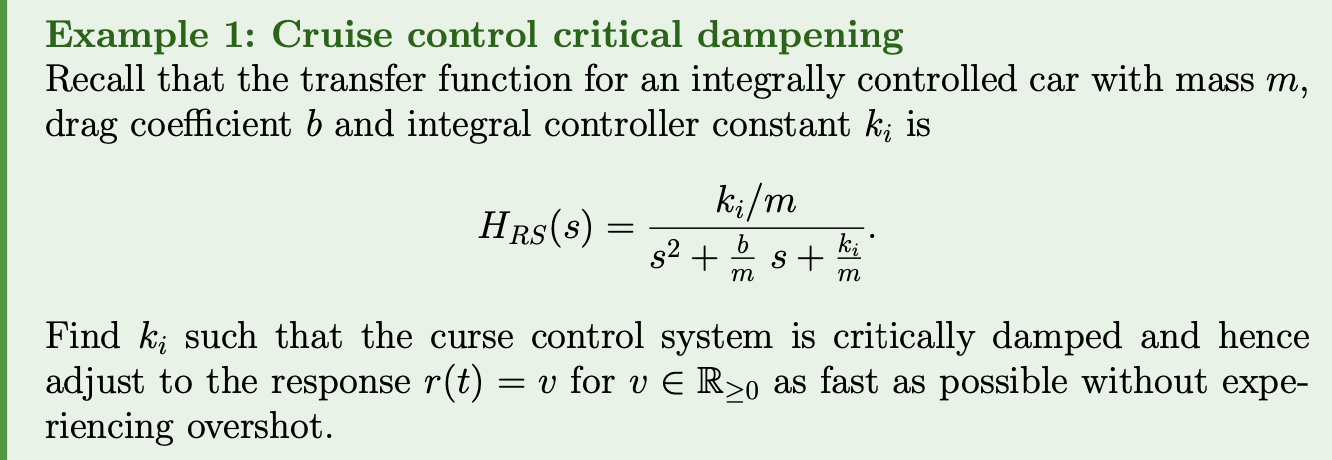
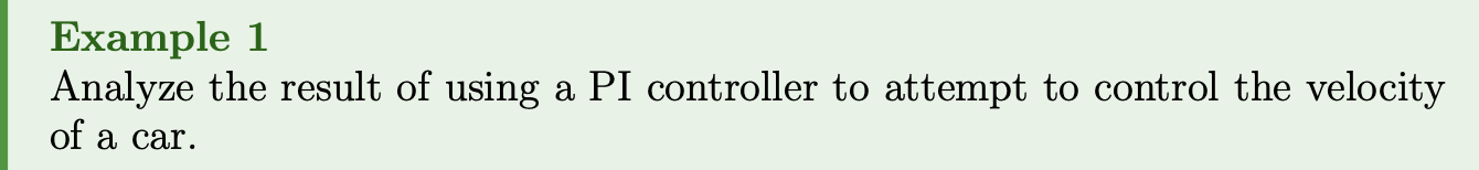
The system diagram for the integrally controlled car cruise control problem from last lecture

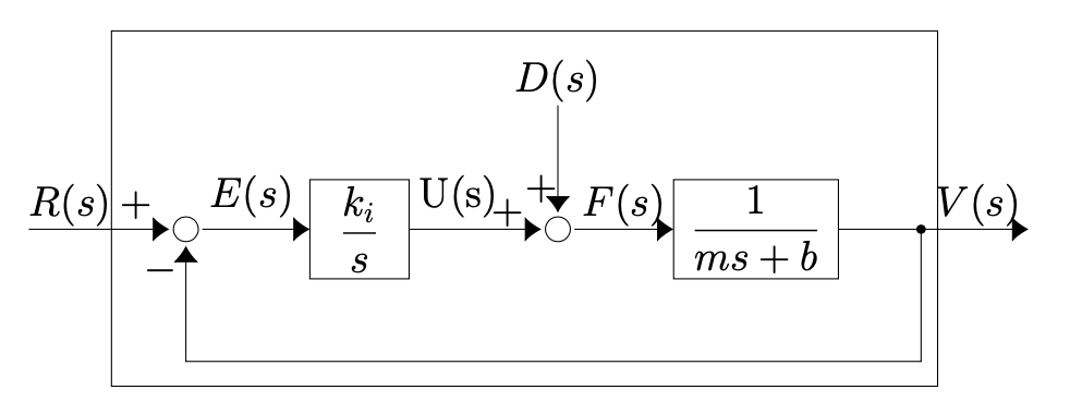
and we found that the transfer function for the controlled system (the big box) is

Do I need to memorize that or is it given in formula sheet??

Systems with transfer functions of this form are common so we will introduce and analyze the standard second order system

Definition 1: Standard second order system

The standard second order system has a transfer function given by

$H(s)=\frac{w^2}{s^2+2\xi ws+w^2}$

where $w>0$ and $\xi \ge 0$.

Examples of theses systems include cruise control with integral control, the harmonic oscillator (with or without damping), and the RLC circuit.

We will now analyze the behaviour of the possible behaviours of the standard second order system. By doing this, we validate the analysis of the cruise control system with an integral controller from the last lecture

The quadratic formula tells us that the poles of $H(s)$ are

$$s_{\pm }=-\xi w\pm w\sqrt{{\xi }^2-1}.$$

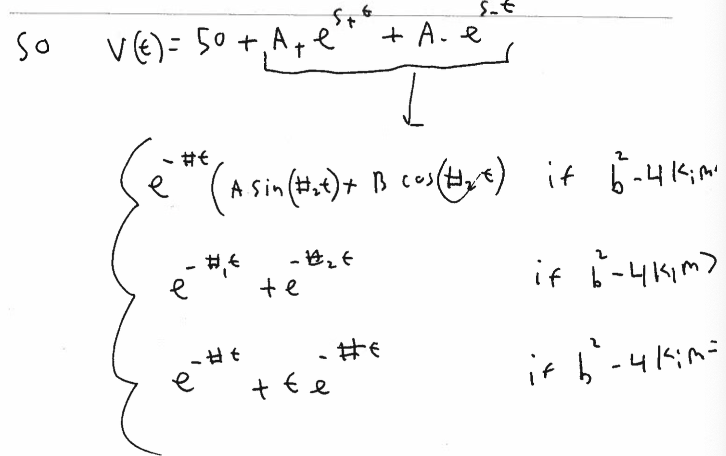
There are hence three different forms of the solution based on where the poles lie.

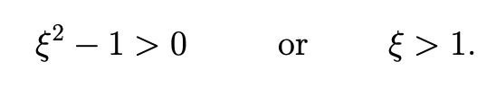
Case 1: Two real distinct pole. (The real roots) In this case $\sqrt{{\xi }^2-1}$ (if $\xi$ is $>0$, then square root $>0$) is real and greater than 0 then there are two distinct real valued poles. (bigger than 0 and a real number)

Since $\xi >0$ for the standard second order system, this happens when

In this case we decompose $H(s)$ via PF as

$$H(s)=\frac{A_{+}}{s-s_{+}}+\frac{A_{-}}{s-s_{-}}$$

for some $A_{+},A_{-}\in \mathbb{R}$.

Thus in this case the standard second order system can be decomposed as sum of two first order systems!!

To show that these are well behaved first order systems (i.e. remain bounded for bounded inputs), first note that for $\xi >1$,

$$\xi >\sqrt{{\xi }^2-1}$$

$\to s-\sqrt{x^2-1}$

Hence,

$$s_{\pm }=-\xi w\pm \sqrt{{\xi }^2-1}$$ $$=w(-\xi \pm \sqrt{{\xi }^2-1})$$ $$<0.$$

Why <0?

To make it have negative real parts?? I guess so

Thus, the poles of the transfer function have negative real parts and therefore any input that is bounded (i.e. has no poles with positive real part) cannot resonate to cause the system response to be unbounded.

For completion, we will find the system’s impulse response. Using the coverup method and simplifying gives

$$A_{\pm }=\frac{\pm w}{2\sqrt{{\xi }^2-1}}$$

and hence the system’s impulse response is

$$h(t)=A_{+}{e}^{s+t}+A_{-}{e}^{s_{-}t}$$

which does decay as $t\to \infty$!

Relating this to A3Q1, this is the overdamped case of the harmonic oscillator

Case 2: One real repeated pole: If ${\xi }^2-1=0$, or simply if $\xi =1$, then there is a single repeated pole at

$$s_{root}=-w.$$

For completion we compute the system is again well behaved.

For completion we compute the system’s impulse response to examine the solution. In this case

$$H(s)=\frac{w^2}{(s-w{)}^2}.$$

Hence the system’s impulse response is simply

$$h(t)=w^{2}t{e}^{-wt}$$

Relating this to A3Q1, this is the critically damped of the harmonic oscillator.

Case 3: Two complex conjugate poles with a non-zero real component: If ${\xi }^2-1<0$, or simply if $0<\xi <1$, then we have complex conjugate poles at

$$s_{\pm }=-\xi w\pm wj\sqrt{1-{\xi }^2}$$

where for ease in future computations, we pulled out the negative from inside the square root.

These roots have negative real parts and hence the system is again well behaved.

We now find the systems’ impulse response. We know that the solution will be decaying sine waves so we prepare the transfer function to use the exponential modulation rule and the sine transform.

$$H(s)=\frac{w^2}{s^2+2\xi ws+w^2}$$ $$=\frac{w^2}{s^2+2\xi ws+w^2}$$

complete the square or just note the roots^

$$=\frac{w^2}{(s+\xi w{)}^2+w^2(1-{\xi }^2)}$$ $$=\frac{w^2}{(s+\xi w{)}^2+(w\sqrt{1-{\xi }^2}{)}^2}$$

from the Laplace Table (LT table) we have

$$h(t)=\frac{w}{\sqrt{1-{\xi }^2}}{e}^{-\xi wt}sin((w\sqrt{1-{\xi }^2})t)$$

I seriously don't know how to compute this with the Laplace Table...

Help, i need the steps

Relating this to A3Q1, this is the underdamped case of the harmonic oscillator.

Case 4: Two complex conjugate poles with a zero real component: If ${\xi }^2-1=0$, or simply if $\xi =0$, then we have complex conjugate poles at

$$s_{\pm }=\pm wj$$

How is this different from case 2??

Isn’t it also ${\xi }^2-1=0$, BUT for case 4, $\xi =0$ and for case 2, $\xi =1$. That’s the difference. Critically damped case $\xi =1$ vs. Undamped case $\xi =0$.

These roots have zero real parts and hence the system may not be well behaved is there is resonance!

We now find the system’s impulse response.

$$H(s)=\frac{w^2}{s^2+w^2}$$

so from the LT table we have

$$h(t)=wsin(wt)$$

Relating this to A3Q1, this is the undamped case of the harmonic oscillator.

We can now plot the impulse response to all these systems. Here is a plot!!

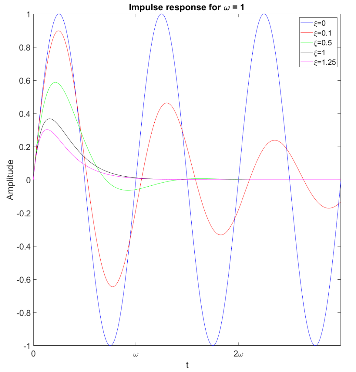
See the L16.m file for a video!

We can also compute the step responses and plot them, we will not show the computations but the step response for $\xi \ge 0$ other than $\xi \ne 1$ is

$$1-\frac{1}{\sqrt{1-{\xi }^2}}{e}^{-\xi wt}sin((w\sqrt{1-{\xi }^2})t+\theta )$$

where $\theta =co{s}^{-1}\xi$. At $\xi =1$ we have a $t$ scaled exponential. Here is a plot of some sample solutions

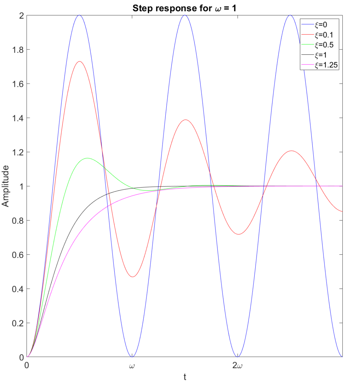
See the L16.m file for a video!

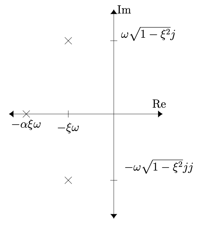
Pole location summary (poles are marked with a $\times$):

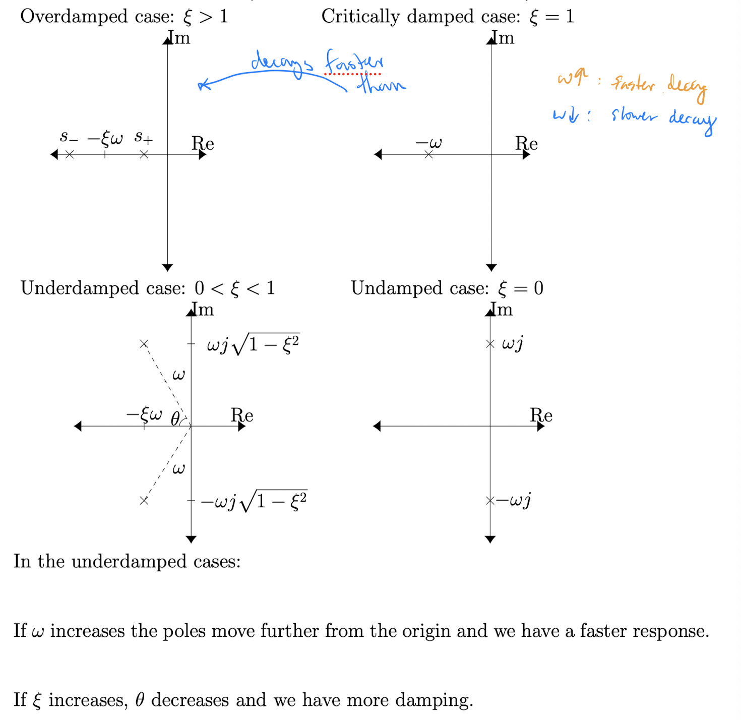
Matlab video!!! See Lecture16.m file for a nice video of the poles and the step response.

Solution: This is a second order system with $w=\sqrt{k_i/m}$ and

$$2\xi w=\frac{b}{m}$$ $$\xi =\frac{b}{2mw}$$ $$=\frac{b}{2\sqrt{m{k}_i}}$$

To be critically damped, we need $\xi =1$ (Case 2) and thus $k_i$ needs to satisfy

$$1=\frac{b}{2\sqrt{m{k}_i}}$$ $$\sqrt{k_i}=\frac{b}{2\sqrt{m}}$$ $$k_i=\frac{b^2}{4m}$$

Here is a plot of the behaviour of the controlled system’s response for values of $k_i$ around this critical value:

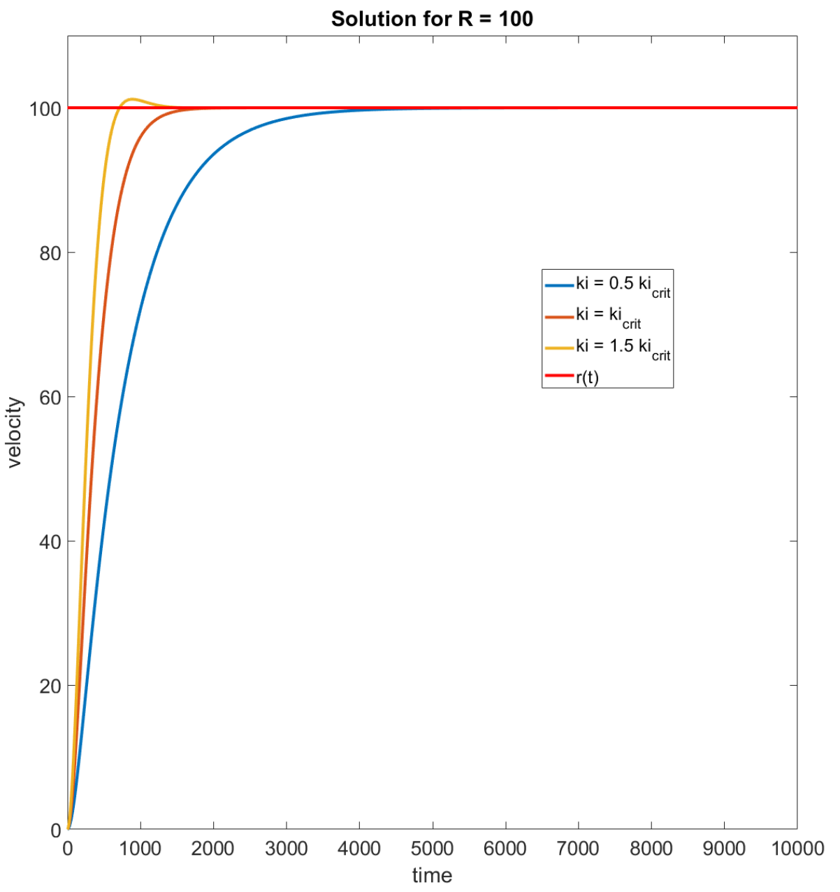
See the second L16.m file if you want to explore this more!

PI controller:

For the cruise control problem, the $P$ controller by itself gets us to a close velocity quickly, but misses the exact velocity and the $I$ controller by itself gets us to the exact velocity, but is slow to do so.

Let’s use them together!!!

The transfer function for this system is

$$H_{RV}(s)=\frac{C(S)S(s)}{1+C(s)S(s)}\leftarrow PreviousResult$$ $$=\frac{(k_p+\frac{k_i}{s})\frac{1}{ms+b}}{1+(k_p+\frac{k_i}{s})\frac{1}{ms+b}}$$ $$=\frac{\frac{k_i}{m}(\frac{k_p}{k_i}s+1)}{s^{2+(\frac{b+k_p}{m})s+\frac{k_i}{m}}}\leftarrow Algebra$$

Next lecture we will analyze this transfer function and how its zeros and poles change the system response and then look at more complex transfer functions.

Lecture 17 - PI controllers, zeros, extra poles and stability

Lecture goals:

• Analyze a PI controller for a first order system
• Know the effects of the zeros and (“extra”) poles of a transfer function

Recall that the system diagram for a PI controlled car is

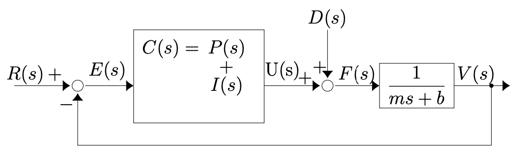
and the transfer function for this system is

$$H_{RV}(s)=\frac{\frac{k_i}{m}(\frac{k_p}{k_i}s+1)}{s^2+(\frac{b+k_p}{m})s+\frac{k_i}{m}}$$

We will first simplify the functional form of $H_{RV}(s)$ to something more familiar by noting that it is of the form

$$H_z(s)=\frac{w^2(\frac{s}{\alpha \xi w}+1)}{s^2+2\xi ws+w^2}$$

where we note that this is almost of the form of the standard second order system but it has a zero.

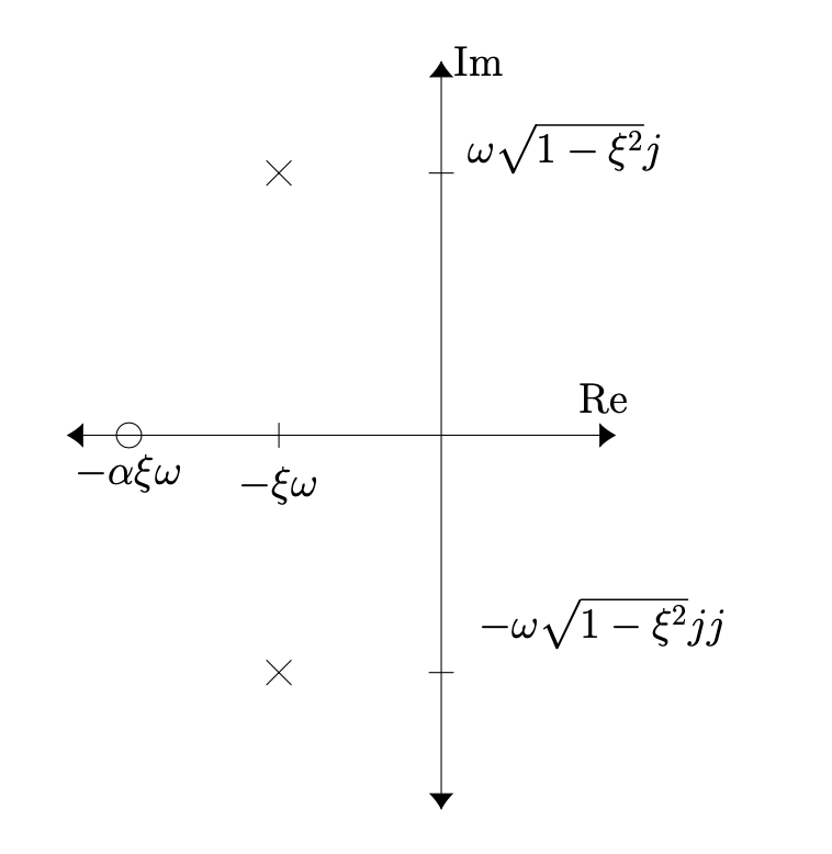
To make the connection between $H_{RV}(s)$ and $H_z(s)$ note that

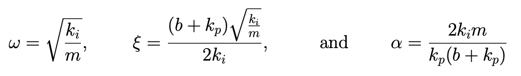
Since $k_i,k_p,b>0$, the poles and zeros can be plotted in the complex plane as

For the cruise control system we mostly care about the step response, so we will analyze the response to the step function.

$$S(u(t))=H_z(s)\cdot \frac{1}{s}$$ $$=(\frac{w^2\frac{s}{\alpha \xi w}}{s^2+2\xi ws+w^2}+\frac{w^2}{s^2+2\xi ws+w^2})\frac{1}{s}$$ $$=\frac{1}{\alpha \xi w}\cdot \frac{w^2}{s^2+2\xi ws+w^2}+\frac{w^2}{(s^2+2\xi ws+w^2)s}$$

This can be decomposed into different responses of the standard second order system

$$S(u(t))=\frac{1}{\alpha \xi w}\cdot \frac{w^2}{s^2+2\xi ws+w^2}+\frac{w^2}{(s^2+2\xi ws+w^2)s}$$

• $\frac{w^2}{s^2+2\xi ws+w^2}$ : Std. 2nd order impulse res.
• $\frac{w^2}{(s^2+2\xi ws+w^2)s}$ : Std. 2nd order step response

We know what the standard second order impulse and step response look like as a function of $w$ and $\xi$ (L16), so we just need to explore how $\alpha$ changes the linear combination of these responses. Since $\alpha$ controls where the zero is, we are studying the effect of the zero on the response.

We will look at the extreme cases:

• If $\alpha \to \infty$ then $S(u(t))\to \frac{w^2}{(s^2+2\xi ws+w^2)s}.$ (Std. 2nd order step response)

In practice, if $\alpha \xi w\gtrsim 10$ then the effects of the impulse response term can ignored in many practical applications.

• If $\alpha \to 0$ then $\frac{1}{\alpha \xi w}\to \infty$. Thus

$$S(u(t))\to \infty .\cdot \frac{w^2}{s^2+2\xi ws+w^2}.$$

and we see a lot of overshooting/instability.

Example

In terms of the cruise control example:

• If $k_p$ increases for a fixed value of $k_i$ then
  • $w=\sqrt{\frac{k_i}{m}}$ is unaffected.
  • $\xi =\frac{(b+k_p)\sqrt{\frac{k_i}{m}}}{2k_i}$ increases. This leads to a faster system response when $\xi >1$ and a slower system response with $0<\xi <1$. It also leads to more oscillations when $\xi <1$.
  • $\alpha =\frac{2k_{i}m}{k_p(b+k_p)}$ decreases. This causes the impact of the standard second order impulse response part of the response to increase. i.e. we will see a larger “bump” in the initial velocity.
• If $k_i$ increases for a fixed value of $k_p$ then
  • $w=\sqrt{\frac{k_i}{m}}$ increases. This in isolation leads to a faster oscillating response.
  • $\xi =\frac{(b+k_p)\sqrt{\frac{k_i}{m}}}{2k_i}$ decreases. This has the opposite effect of $k_p$.
  • $\xi =\frac{(b+k_p)\sqrt{\frac{k_i}{m}}}{2k_i}$ increases. This has the opposite effect of $k_p$.

Generally, for this application we care about getting to the steady state velocity quickly and do not want to overshoot. Hence we want no oscillations and we want the impact of the impulse term to not cause overshooting.

Combining the effects above,

for this system we use $k_i$ to adjust the speed of the response and $k_p$ to control the dampening of the oscillations. The exact values of $k_i$ and $k_p$ needed will depend on $b$ and $m$ but generally we want $\xi >1$ to avoid the oscillations.

todo Review this again

Didn’t really understand…

See the Lecture17_PI_controller.m for some examples of the controlled velocity.

Adding a pole:

Since $k_i,k_p,m,b>0$, the poles and zeros can be plotted in the complex plane as

Based on the locations of the poles/functional form of $H(s)$ we note that we can decompose $H(s)$ as a linear combination of first and second order systems

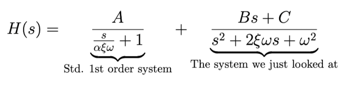
We need to know the relative values of $A,B,C$ (and the decay rates of the system responses) to know what the impulse response looks like.

Evaluating the PF decomposition components givestodo

Understand and learn how to do this.

I forgot…

$$A=\frac{1}{1-2\alpha {\xi }^2+{\alpha }^2{\xi }^2}$$ $$B=\frac{-\alpha \xi w}{1-2\alpha {\xi }^2+{\alpha }^2{\xi }^2}$$ $$C=\frac{\alpha (\alpha -2){\xi }^2{w}^2}{1-2\alpha {\xi }^2+{\alpha }^2{\xi }^2}.$$

$\alpha$ changes the relative weights of the impacts of the first order system and the second order system. What happens as $\alpha$ changes?

We again look at the extreme values:

• If $\alpha \to 0$ then $A\to 1$ and $B,C\to 0$.

In this case, the impulse response looks like that of a standard second order system given that the complex poles are closer to the imaginary axis than the complex pole.

The latter happens when $-\alpha \xi w>-\alpha w$. In practice this happens for $\alpha \lesssim 0.1$ or so.

• If $\alpha \to \infty$ then $A,B\to 0$ and $C\to w^2$.

In this case, the impulse response looks like that of a standard second order system given that the complex poles are closer to the imaginary axis than the real pole.

Assuming the roots are complex valued (i.e $0<\xi <1$), the latter happens when $-\alpha \xi w<-\xi w$. In practice this happens for $\alpha \gtrsim 10$ or so. If the roots are not complex then the second order system decomposed into two first order systems but the result still holds.

See Lecture17_extra_poles.m for pictures showing this.

Definition 1

When a real pole or a complex-conjugate pair of poles are an order of magnitude closer to the imaginary axis than all other poles then we say that they are dominant.

Dominant pole

Pick the dominant poles and ignore the others in order to determine the behaviour.

Linear Stability:

Recall the general behaviours of the impulse response caused by a pole at some point $a+bj$ for $a,b\in \mathbb{R}$.

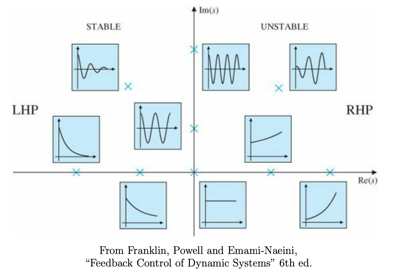
The impulse response of ALL Linear Time Invariant systems is a linear combination of the types of functions shown in the above plot. ($\to$ because of PF)

Further since $\{\delta (t-\tau )|\tau \in \mathbb{R}\}$ is a basis for the set of all functions, the response of ANY LTI to ANY function $f(t)$, can be written as a convolution of $f(t)$ with a linear combination of the types of functions shown above.

Definition 2: System Stability

LTI, $S$, is stable if $S(\delta (t))$ decays to 0.

A LTI, $S$, is unstable if $S(\delta (t))$ is unbounded.

A LTI, $S$, is marginally stable if $S(\delta (t))$ is bounded but does not decay to 0. (sin, cos)

The type of stability mentioned above is often called linear stability.

Definition 3: Transfer function stability

A transfer function is stable if the system it is a transfer function for is stable.

A transfer function is unstable if the system it is a transfer function for is unstable.

A transfer function is marginally stable if the system it is a transfer function for is marginally stable.

Theorem 1: Stability

A transfer function is stable if all poles have a negative real part.

A transfer function is unstable if there is a pole with a positive real part OR there is a second order pole that has a real part of 0. (but if pole of first order, then it is marginally stable)

A transfer function is marginally stable if there are no poles with positive real parts OR second order poles with a real part of 0 and in addition there is at least order 1 pole that has a real part of 0. (can have pole on imaginary 0, but they need to be first order)

Sketch of proof:

If all poles have negative real parts then the impulse response is a sum of exponentials (potentially with oscillations) that decay to 0 and hence the impulse response decays.

If there is any pole with a positive real part, then that component of the impulse response grows. Hence the impulse response will not be bounded.

If the first condition is met, then the system is not unstable and hence the impulse response does not grow without bound. If the second condition is met then there is either a sinusoidal component to the impulse response or a constant component. In either case, these terms will keep the system response from decaying to 0.to-understand

Definition 4: Bounded-input, bounded-output (BIBO) stable

A LTI, $S$, is bounded-input, bounded-output (BIBO) stable if $S(f)$ is bounded for all bounded functions $f$.

Theorem 2

A LTI system with a rational transfer function is BIBO stable if and only if its transfer function is both stable and proper.

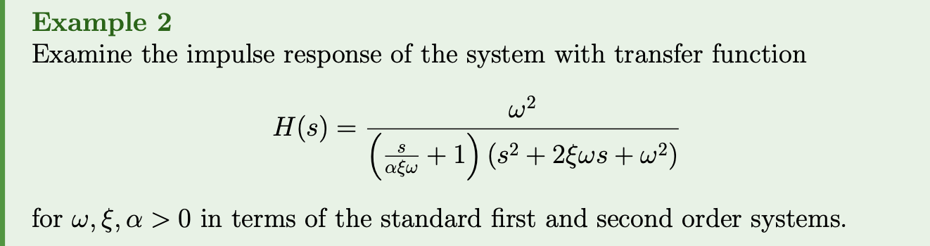
Example 3

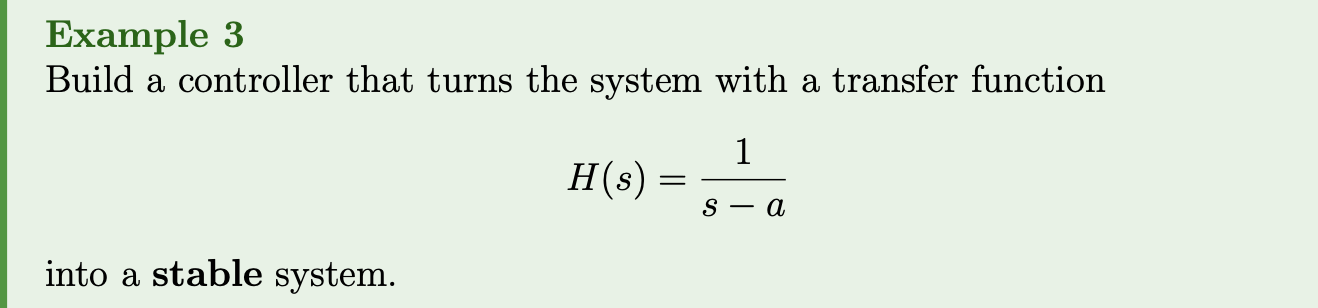
Assume $a>0$.

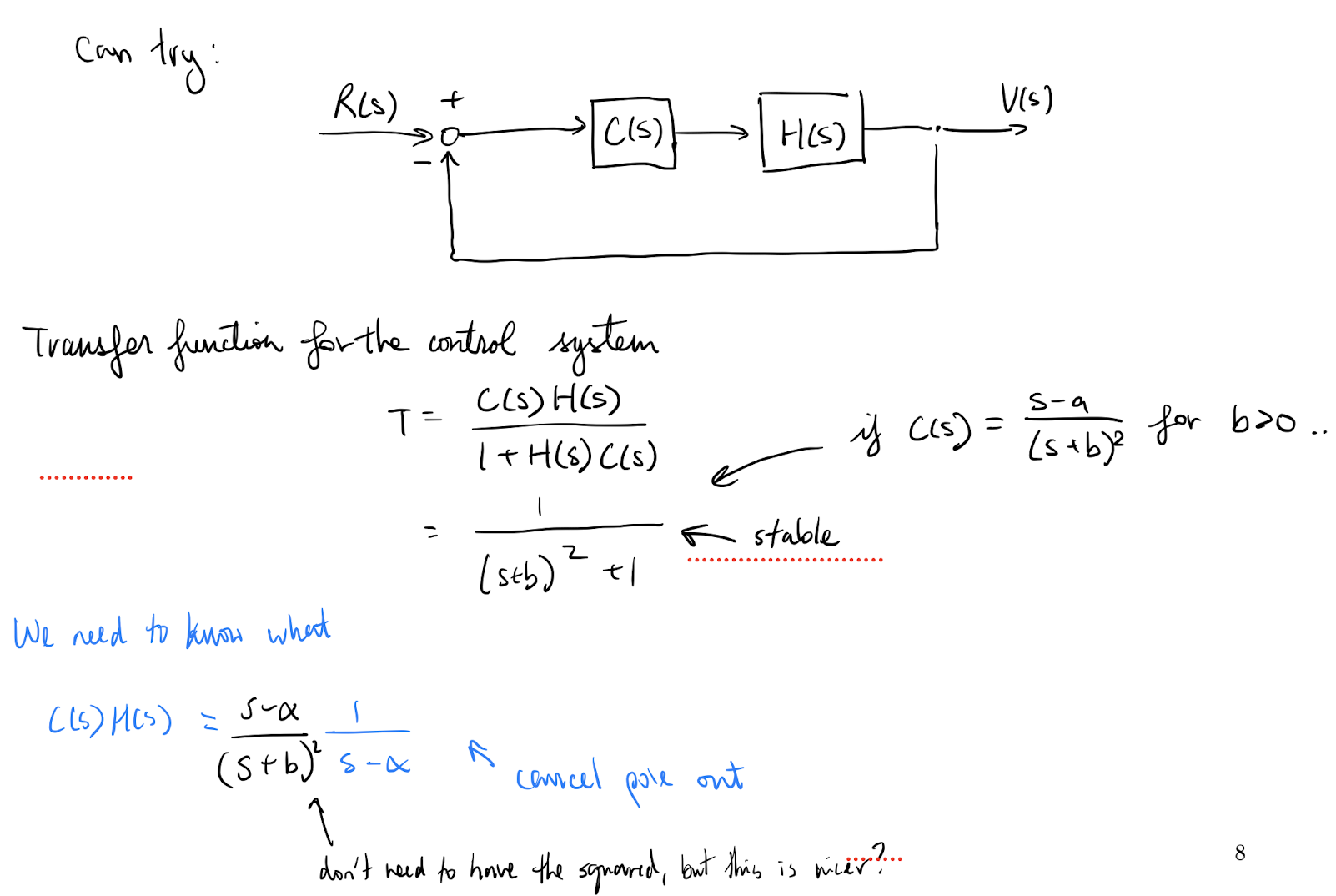
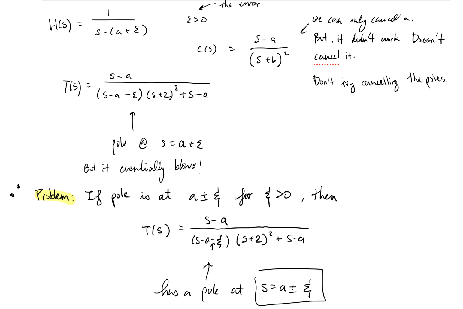
Understand this problem.

And wtf is T (transfer function) that we got? Where did we get it from?

Why is $C(s)=\frac{s-a}{(s+b{)}^2}$ for $b>0$???

Why is it stable? Look at the definitions.

NASA tried this method for a Jupiter rocket (1957) and Atlas 4a rocket (1957) and others… don’t do this!

I repeat NEVER cancel unstable poles in the above way. Go to the tutorial if you want to see how to do this properly.

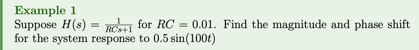
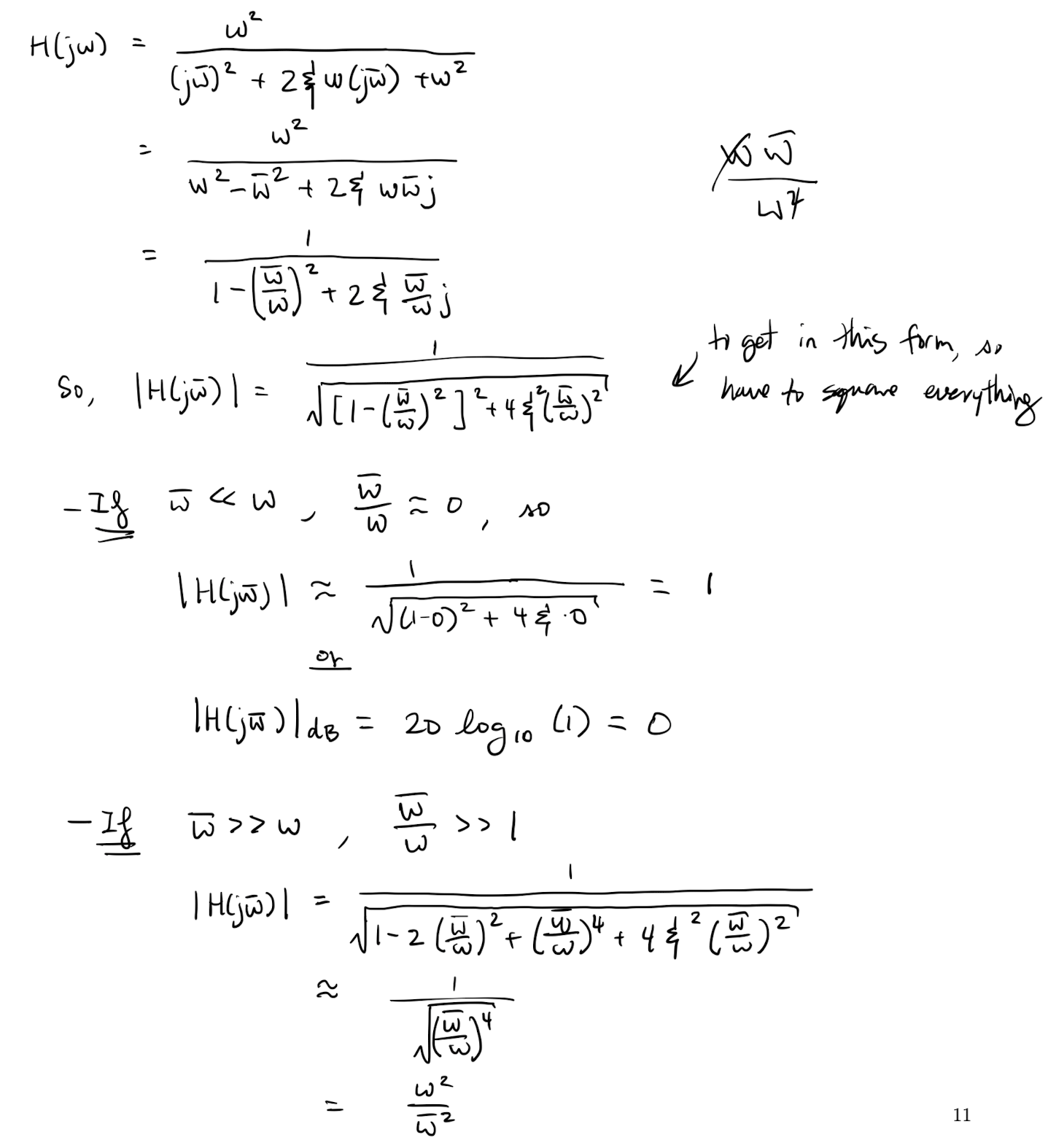
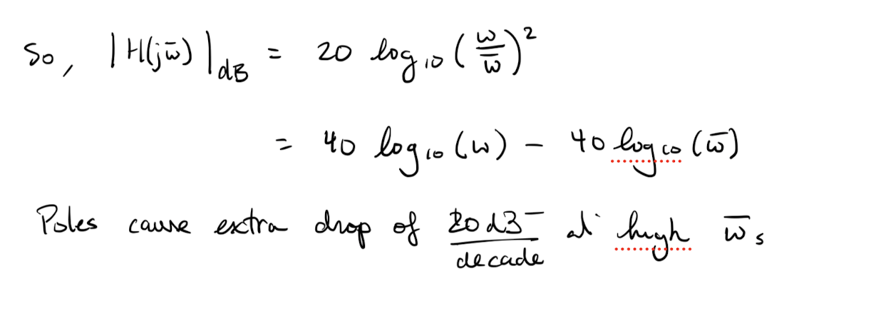
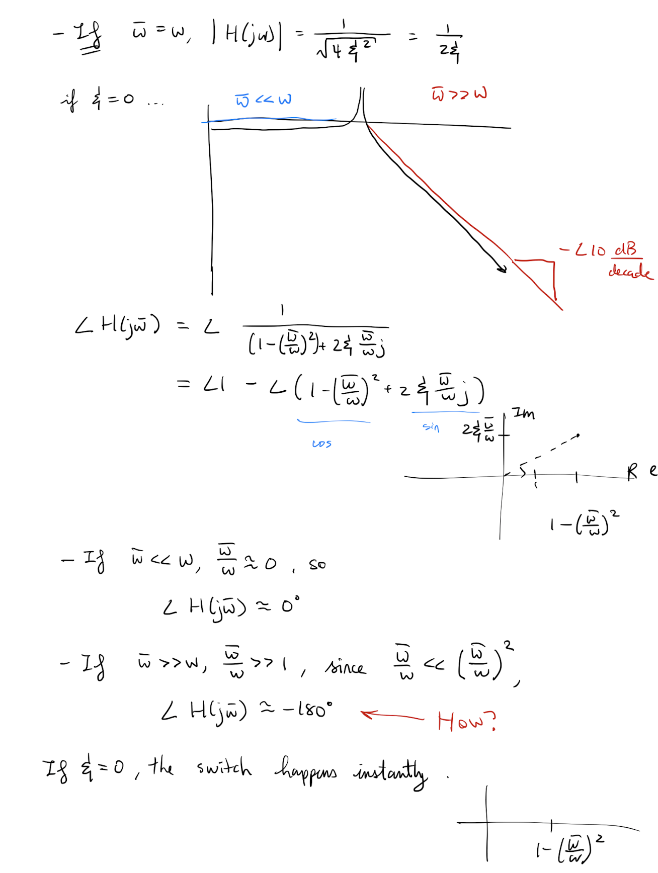
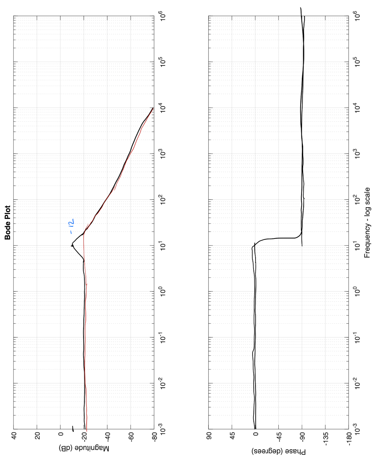
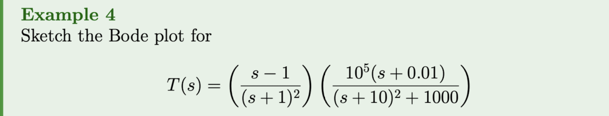
Lecture 18 - Bode plots

Lecture goals:

• Understand what the frequency response is and
• be able to generate and interpret Bode plots.

In lectures 13-17 we learned how to:

• compute the response of a LTI given an input function $f(t)$ by either evaluating ${\mathcal{L}}^{-1}\{H(s)\}\ast f(t)$ or computing ${\mathcal{L}}^{-1}\{H(s)F(s)\}$,
• analyze the general structure of the unit impulse and step responses by looking at the poles (and zeros) of the transfer function
• apply simple control systems (P, I, and PI) to control a system to have the behaviour we want it to have (i.e. cruise control problem).
• that the transfer function is the Laplace transform of the system’s impulse response
• that complex exponentials are the eigenfunctions of LTIs

These methods work well for many simple/academic problems but this method requires us either to find all of the poles (or potentially the dominant ones) or to evaluate a convolution integral.

Sometimes it is not possible to find all the poles/roots of the transfer function!

Sometimes we want to work in the time domain rather than the frequency domain.

In these cases, we need to use a different approach that has its own pros and cons.

Deriving the frequency response:

Recall Theorem 4 from lecture 13:

Theorem 1: LTI response to an exponential

If $S:f\to y$ is a LTI with transfer function $H(s)$ then for an $s\in \mathbb{C}$

$e^{st}\to H(s)e^{st}$.

Now, if $s=jw$ then the above gives $e^{jwt}\stackrel{S}{\to }H(jw)e^{jwt}$.

$H(jw)$ is a complex number so we can “recall” from MATH115 that we can write it in polar form:

$$H(jw)=|H(jw)|e^{j{\angle }_{H(jw)}}$$

“Recall” from MATH115 that this decomposition can be viewed geometrically:

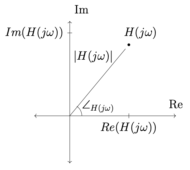
Now we can write the system’s response to $e^{jwt}$ as

$$H(jw)e^{jwt}=|H(jw)|e^{j{\angle }_{H(jwt)}}{e}^{jwt}$$ $$=|H(jw)|e^{w+{\angle }_{H(jw)}jt}$$

• $|H(jw)|e^{j{\angle }_{H(jwt)}}$: $H(s)$

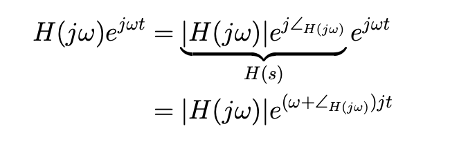
Because of the above, $H(jw)$ is called the frequency response.

Explicitly, $H(jw)$ is the factor we need to scale the input signal $e^{jwt}$ by in order to find the system’s response of $e^{jwt}$.

Theorem 2

If $S$ is a LTI with transfer function $H(s)$, then

$sin(wt)\stackrel{S}{\to }|H(jw)|sin(wt+{\angle }_{H(jw)})$

Sketch of proof: Recall that

$$sin(wt)=\frac{e^{jwt}-e^{-jwt}}{2j}$$

Use the above identity along with the previous results and then do some algebra.

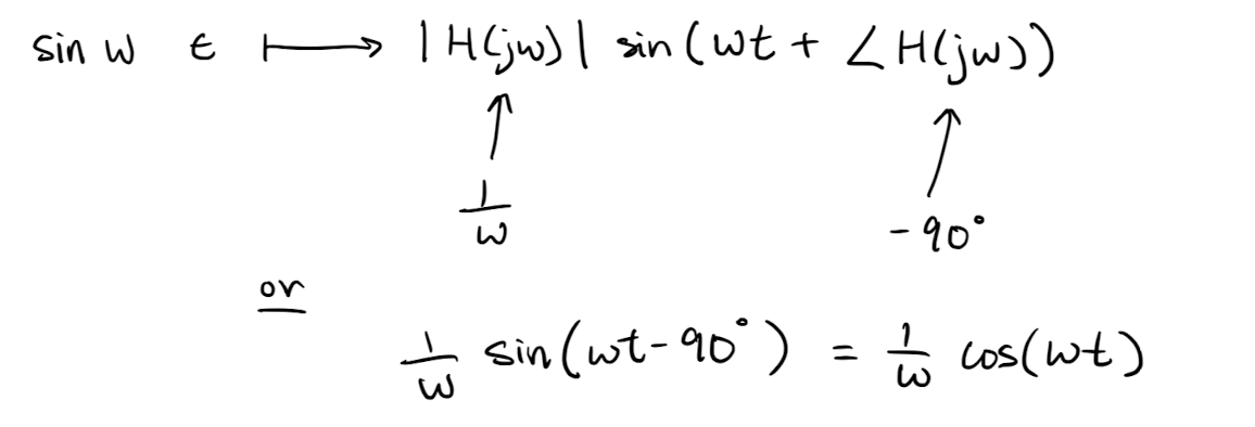
Observations: The above says that the system response of an LTI to a sin wave of frequency $w$:

• has an amplitude scaled by $|H(jw)|$
• has the same frequency
• Has a phase shifted by ${\angle }_{H(jw)}$

In the real world signals have a clear starting time (i.e. real world signals are one sided) so the above can’t be used for many applications. Lucky for us:

Theorem 3

If $S$ is a stable LTI with transfer function $H(s)$, then as $t\to \infty$

$sin(wt)u(t)\stackrel{S}{\to }|H(jw)|sin(wt+{\angle }_{H(jw)})$.

We will skip this proof.

Looking ahead: Fourier series/transforms will allow us to decompose functions as a sum/integral of sin and cos waves.

Hence if we know what the LTI does so all complex exponentials, then we can decompose a signal into a sum/integral of complex exponentials, scale and phase shift them, and then add the results together to see the response to the original signal.

We want a nice way to display the scaling factors and phase shifts so we introduce Bode plots.

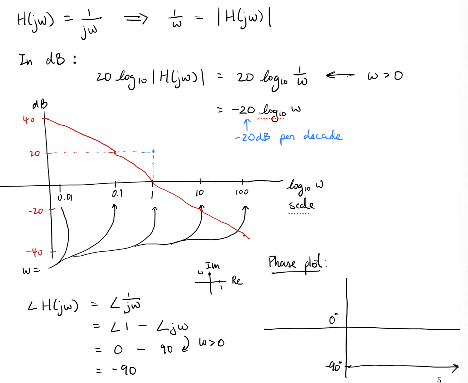
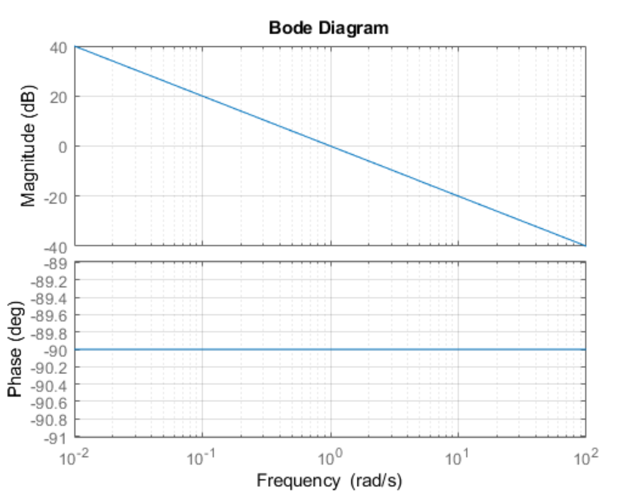
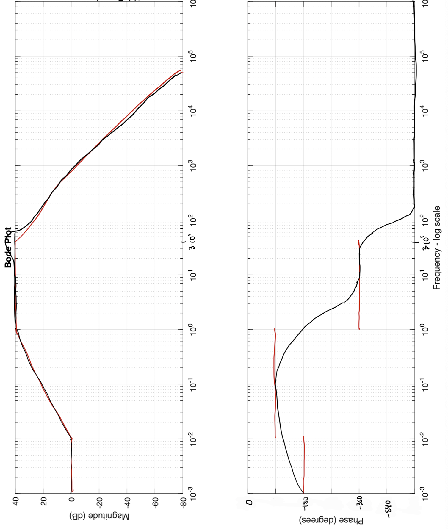
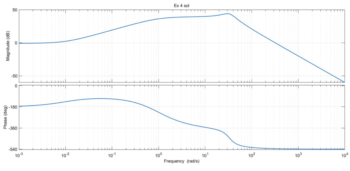
Bode plots:

• Bode plots re a graphical representation of the frequency response.
• We need two plots: one for $|H(jw)|$ in “decibels” (dB) vs ${\log }_{10}(w)$ and one for $\angle H(iw)$ vs ${\log }_{10}(w)$
• The aforementioned plots are called the “magnitude” and “phase” curves respectively.

Using these conventions has two benefits:

• it allows curves to be approximated by piecewise lines (we will show this via examples).
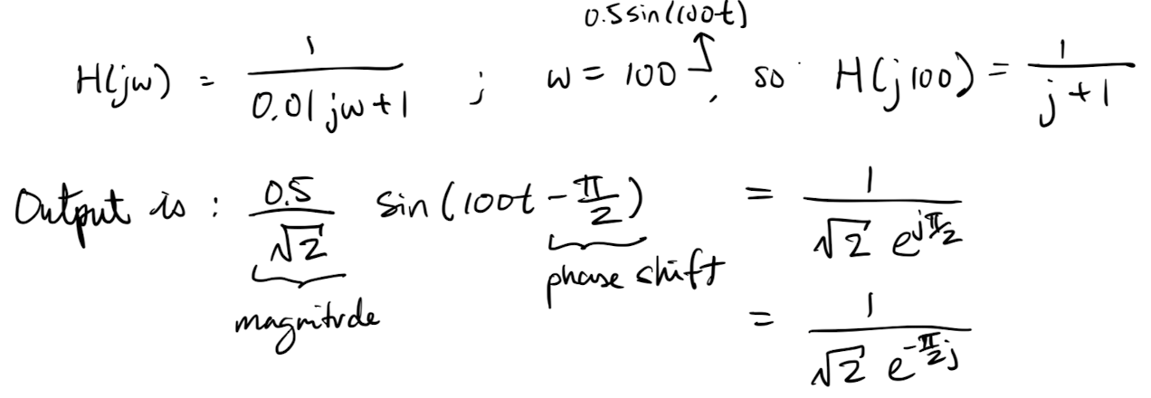
• allows plots for complex transfer functions to be build by adding plots from simpler transfer functions.

To see the basic idea behind this approach suppose $H(jw)=H_1(jw)H_2(jw)$ and that we have the Bode plots for $H_1$ and $H_2$.

In this case:

The angles are additive so we can simply add the phase curves of $H_1$ and $H_2$ to get the phase curve for $H$.

The magnitudes are not additive but… “recall” that $\log (ab)=\log (a)+\log (b)$ so if we use decibels for the magnitude, then the magnitude curves become additive.

Definition 1: Decibels

$|H(jw)|$ in decibels is $20{\log }_{10}(|H(jw)|)$.

Using decibels for the magnitude: if $H(jw)=H_1(jw)+H_2(jw)$ then we have

$$20{\log }_{10}(|H(jw)|)=20{\log }_{10}(|H_1(jw)|)+20{\log }_{10}(|H_2(jw)|).$$

So if we use decibels, then we can just add the magnitude curves to find the magnitude curve of $H(jw)$.

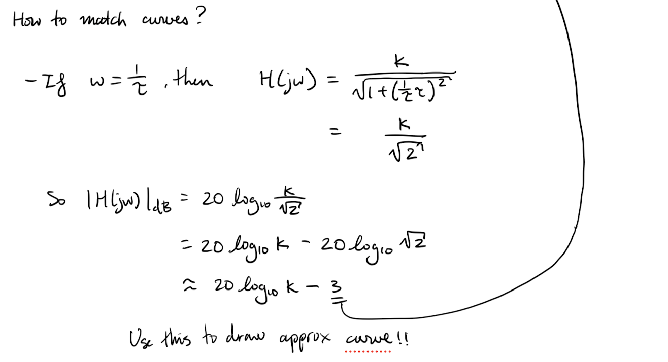
Bode plot examples:

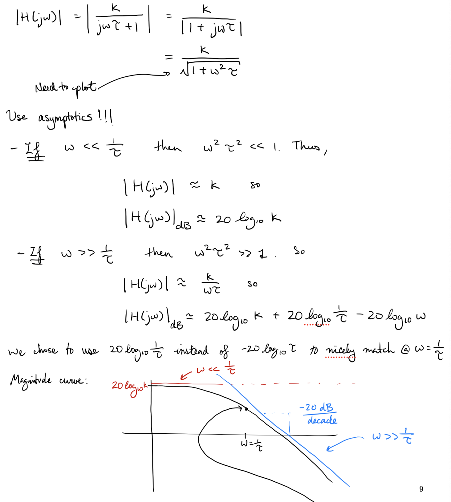
Some questions I have (should've attended class):

• How is $\angle \frac{1}{H(wj)}=\angle 1-\angle H(wj)$??

From ChatGPT

For understanding why $\angle \frac{1}{H(jw)}=-\angle H(jw)$ in the context of Bode plots, we need to consider the properties of complex numbers and their representation in polar form.

Given that $H(jw)=|H(jw)|e^{j\angle H(jw)}$, where $|H(jw)|$ represents the magnitude of $H(jw)$ and $\angle H(jw)$ represents its phase angle, we can write $\frac{1}{H(jw)}$ as:

$\frac{1}{H(jw)}=\frac{1}{|H(jw|}{e}^{-j\angle H(jw)}$

Now, let’s examine the phase angle of $\frac{1}{H(jw)}$. According to Euler’s formula, $e^{-j\theta }$ represents a rotation in the complex plane by an angle of $\theta$ in the clockwise direction. Therefore, if $H(jw)$ has a phase angle of $\theta$, $\frac{1}{H(jw)}$ will have a phase angle of $-\theta$.

In other words, $\angle \frac{1}{H(jw)}=-\angle H(jw)$.

This property is important in Bode plots because when plotting the phase response, the phase of $\frac{1}{H(jw)}$ is essentially the negative of the phase of $H(jw)$, which affects the overall behaviour of the system at different frequencies.

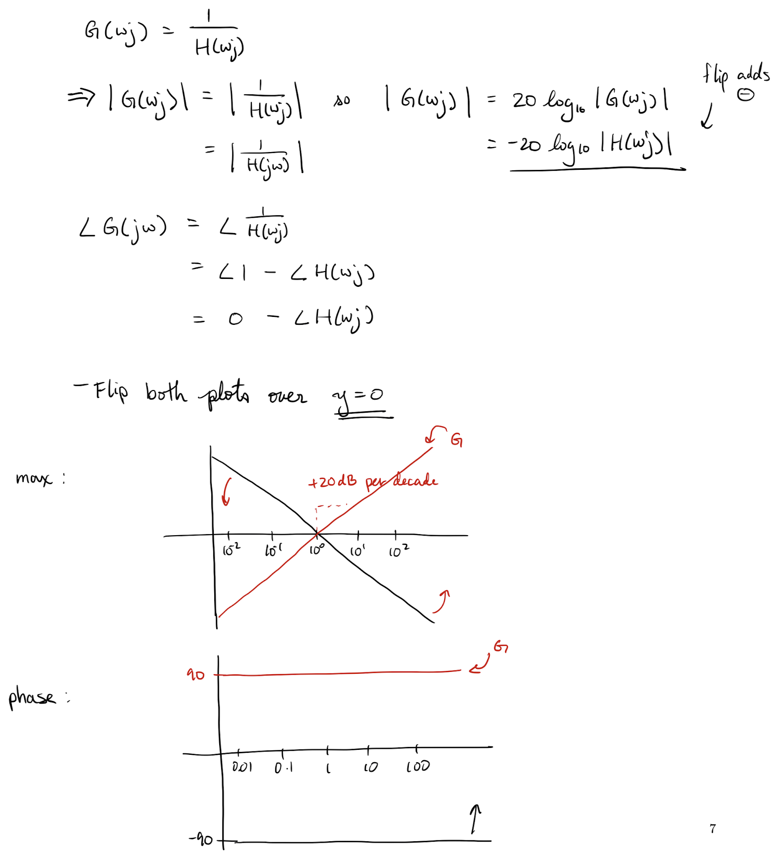
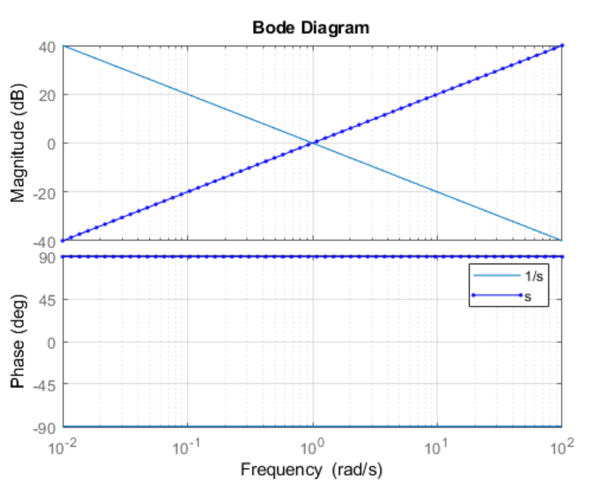
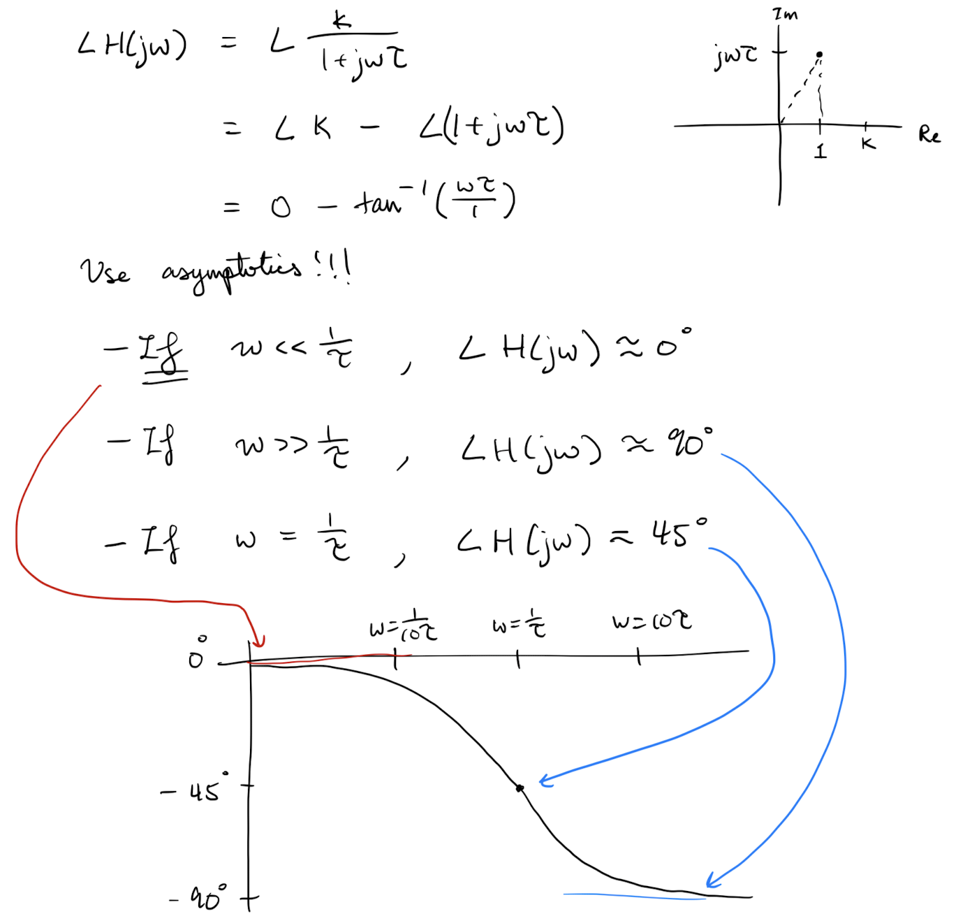
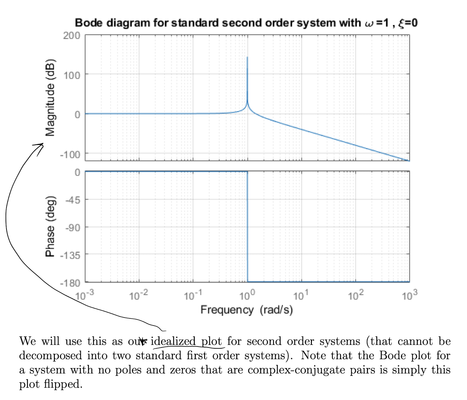
Note that the Bode plot for a system with no poles and a zero is simply this plot flipped over $y=0$.

Thinks I dont understand about this example's solution

• Why use $\bar{w}$?
• For if $\bar{w}>>w$, $\frac{\bar{w}}{w}>>1$, why is $|H(j\bar{w})|$ the way it is? In denominator…
• How did it simplify to $\frac{1}{\sqrt{(\frac{\bar{w}}{w}{)}^2}}$?
• How did we get $-180^o$?

If a given a transfer function $H(s)=H_1(s)\cdot H_2(s)\cdot \cdot \cdot H_k(s)$ then the Bode plot for $H(jw)$ is found by

• Finding the magnitude and phase curves for each $H_i(jw)$.
• Adding the magnitude and phase curves

Lecture 19 - Bode plots 2

Lecture goals:

• Refine our ability to quickly draw bode plots,
• approximate the transfer function from bode plots,
• and determine stability of the system/closed loops using Bode plots.

Summary of main results from Lecture 18:

• The “starting value” of the magnitude curve is $|H(0){|}_{dB}$ and the “starting value” of the phase curve is $\angle H(0)$.

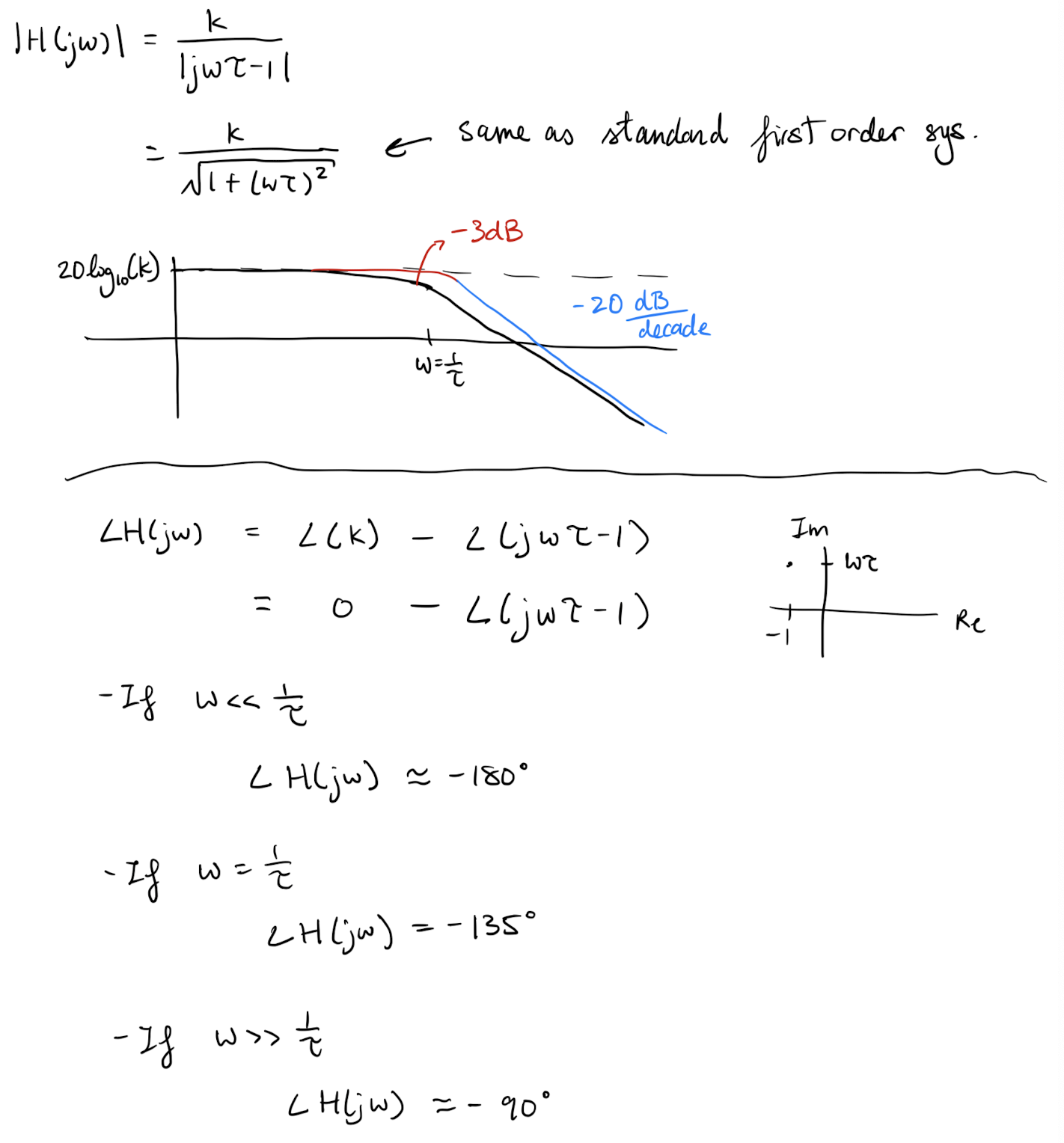
  This will be not exists (i.e. the curve is unbounded) if there is a pole with a real value of 0.

• If the transfer function has an order one stable pole at a point then the magnitude curve will experience an extra decrease of $-20dB/Decade$ and the phase curve will experience a drop of $-90^o$ (see L18 Ex 4).

  These phase adjustment will be rather “slow” taking an order of magnitude (before and after the pole) to adjust.

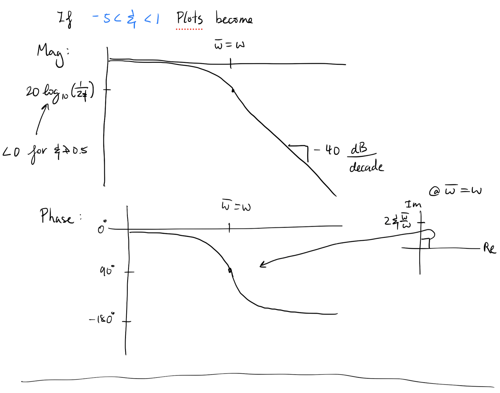
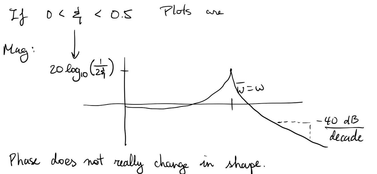
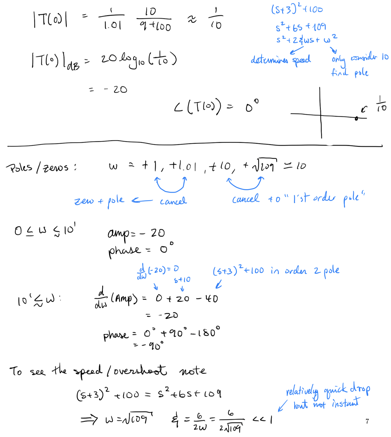
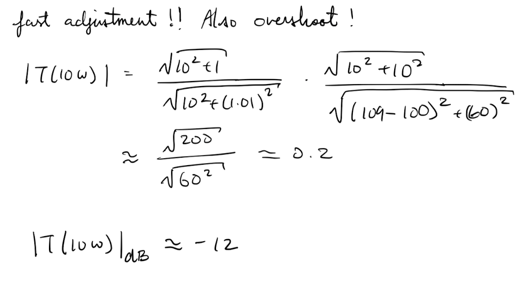
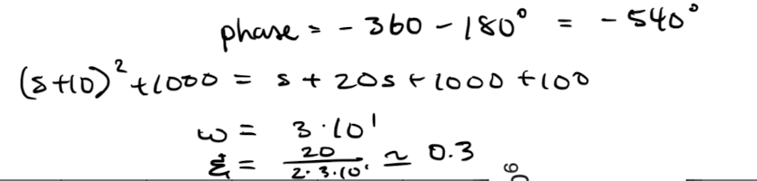
• If the transfer function has complex conjugate poles that are stable then the magnitude curve will experience an extra decrease of $-40dB/Decade$ and the phase curve will experience a gain of $-180^o$. The location of this adjustment is given by $w$ is the term in the standard second order system (see L18 Ex 5).

• The speed of adjustment is related to $\xi$:

  • $\xi \approx 0$ causes fast adjustments and overshooting in the amplitude plot for nearby $ws$,
  • $\xi \approx 1$ causes slow adjustments and undershooting in the amplitude plot for nearby $ws$.

• If we have zeros of order 1 or of order 2, at some point then the magnitude and phase curves experience the opposite effects as listed in the above two points.

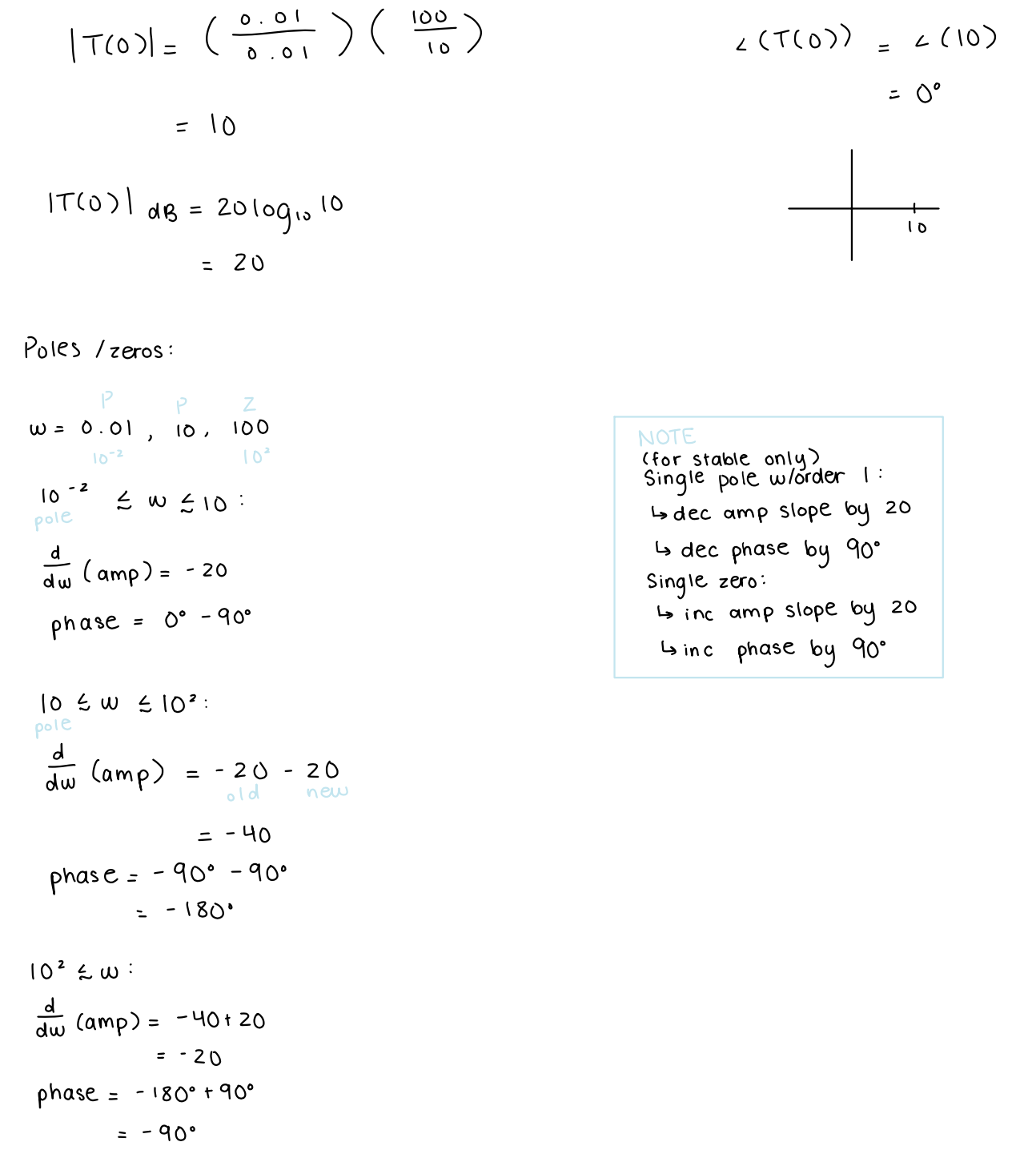
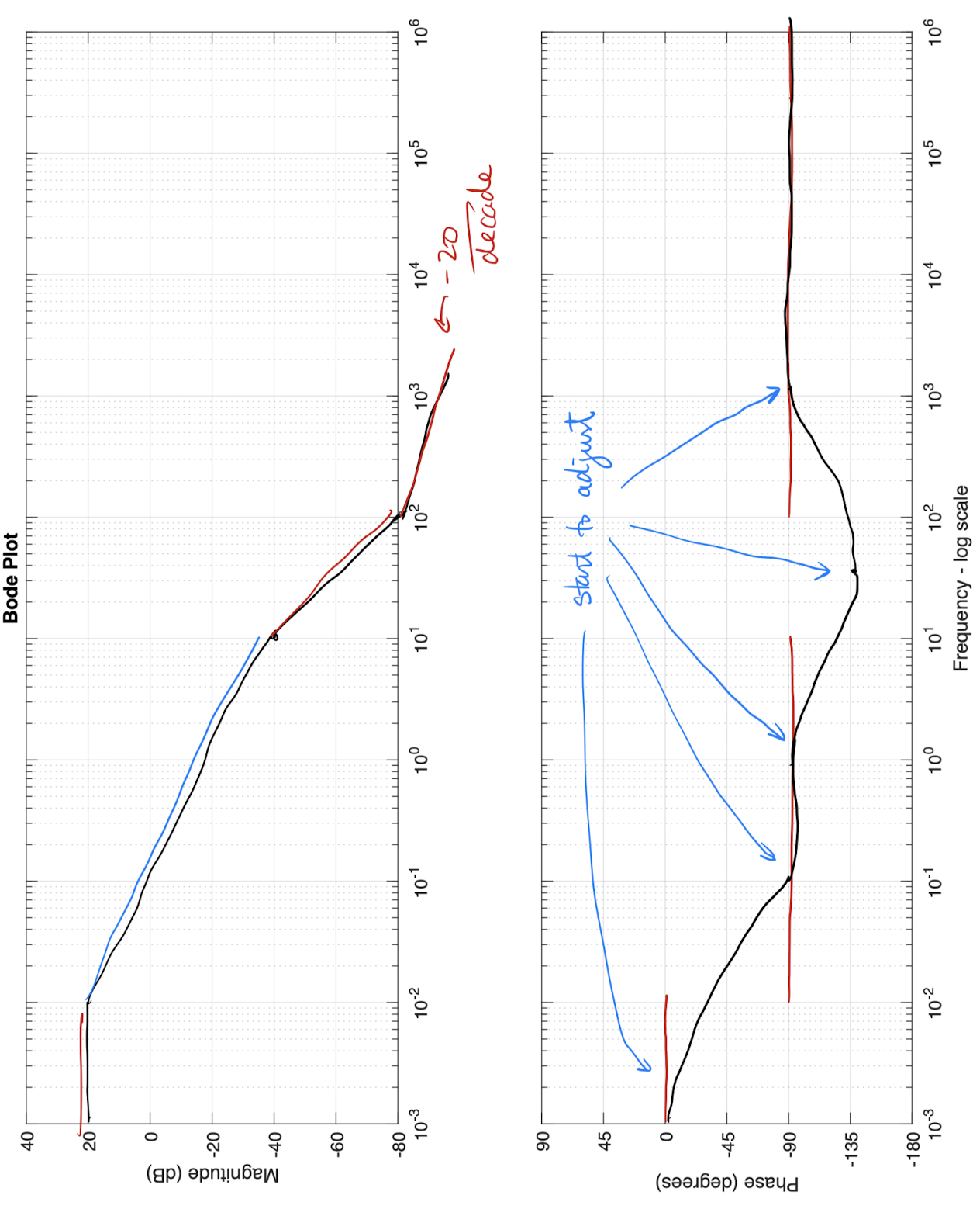
What if we have an unstable pole?

In this case Bode plots do not make sense to apply as they assume there is a steady solution but… for completion

$H(s)=\frac{\kappa }{s\tau -1},\kappa ,\tau >0$

Similar result for second order systems but they are a bit more complex to analyze and often there are better ways to test stability so we skip the analysis.
In general if you see a decrease in the slope of the asymptotic amplitude curve and an increase in the phase, then you can conclude that the system is unstable (and hence a Bode plot should have never been made). You can not conclude anything about stability of the system modelled by the transfer function used to generate the plot though.

To quickly generate plots, we can use the results derived from lectures 18 and 19 by either adding the curves or using the relation of the poles/zeros and the curves to sketch asymptotic lines. The latter is often nicer.

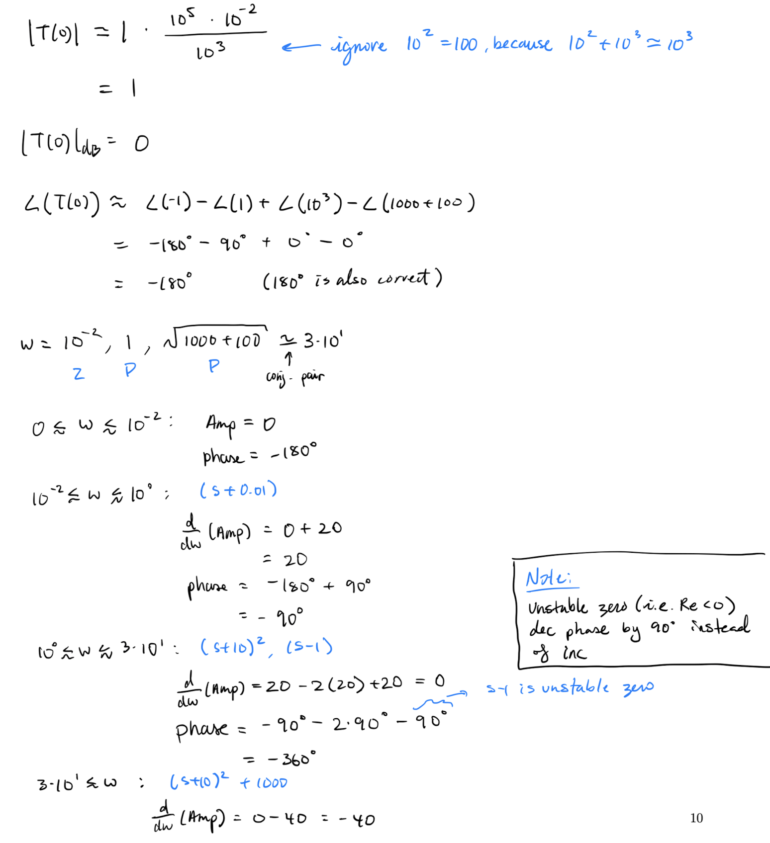
Note

Unstable poles (dec net amp change + inc phase) make system unstable. Unstable zeroes don’t, but can cause more oscillations.

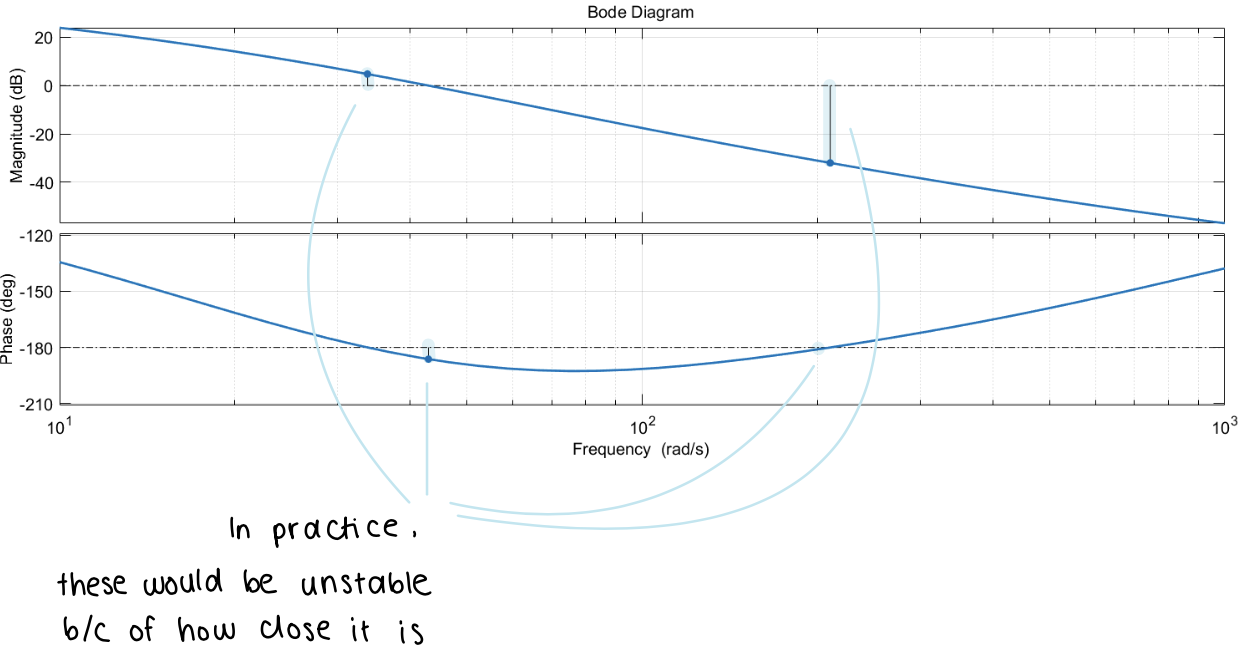
Recall that for a closed loop system with system diagram given by:

The transfer function for this system is

$$\frac{P(s)C(s)}{1+P(s)C(s)}$$

Hence the closed system will be stable when both $C(s)$ and $P(s)$ are stable and when

$$1+P(s)C(s)\ne 0.$$

Hence if $C(s)$ and $P(s)$ are both stable, then the closed loop control system is unstable when

$$P(s)C(s)=-1$$ $$=1\cdot e^{i\pi }.$$

This happens when the amplitude curve is $|1{|}_{dB}\approx 0$ while the phase is either $180^o$ or $-180^o$ (or some other equivalent angle).

In general to talk about stability we will not look for these exact conditions but will instead look at the points where either the amplitude or the phase is critical and then look at how far we are from stability. We generally require some threshold to be “far enough” from being unstable.

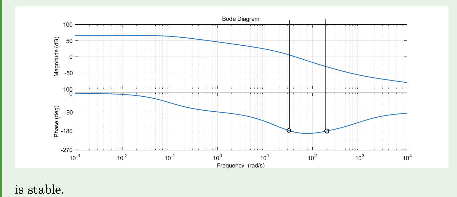
Formally stable, but close to unstable.

Lecture 20 - Signals - Intro

Lecture goals:

• know the big picture of Fourier series/transforms

Bode plots allows us to quickly see how a system responds to input signals of the form $sin(wt)$.

This can be used to quickly tell what type of filtering/amplifying the LTI does to the sin wave.

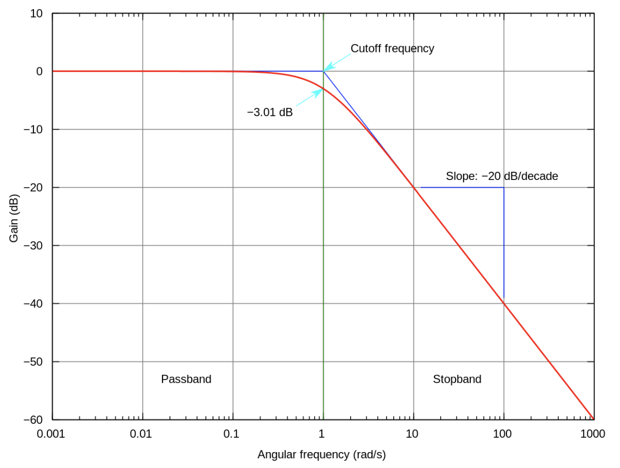
For example a low pass filter is a LTI that removes the “high” frequency waves. Explicitly, they reduce the amplitude of all waves with a frequency larger than some cutoff $w$.

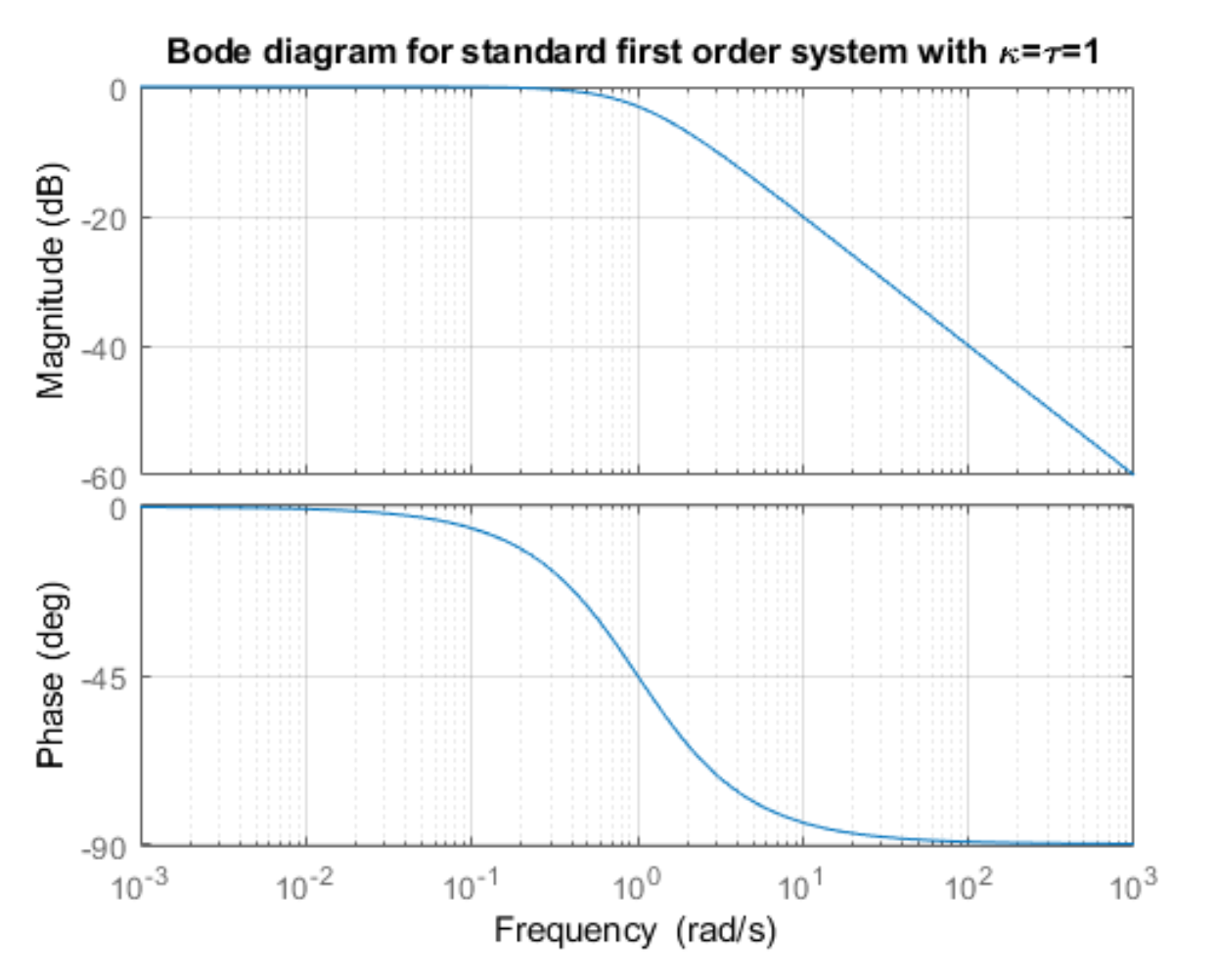
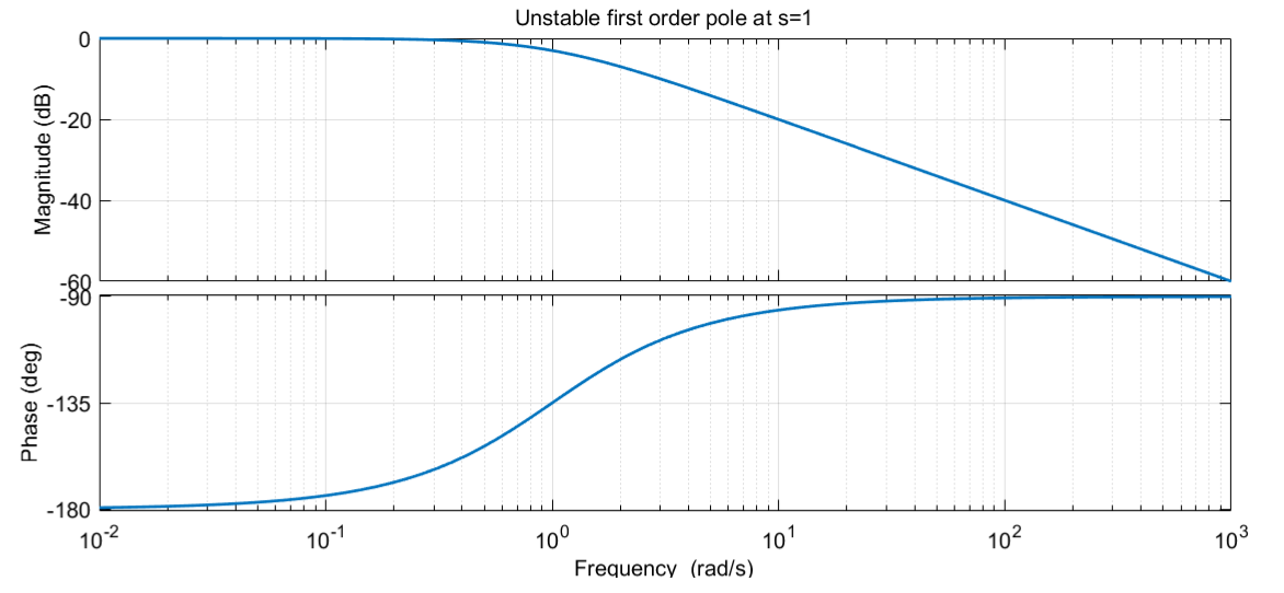
All stable systems with a single pole and no zeros are low pass filters. Here is the hopefully familiar amplitude plot (stolen from wiki because I liked their annotations):

$1=T(s)=\frac{1}{s+1}$

As another example for a high filters we need the amplitude curve to go to $0$dB at some cutoff point. The standard high pass filter transfer function is

$$T(s)=\frac{as}{s+w_0}$$

for $a,w_0>0$ and its bode plot is

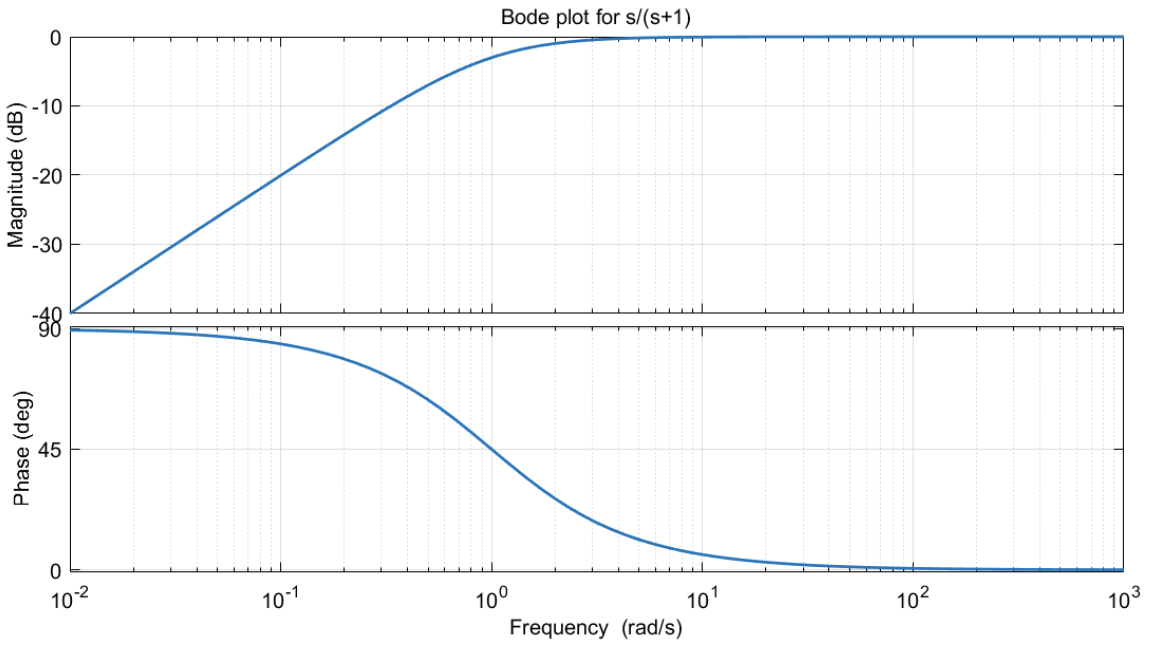
If you wanted stronger drops in the frequency, you could simply add more zeros near 0 and poles to counter them!!!

If you wanted a medium band filter, then you can add another pole later:

$$T(s)=\frac{as}{(s+w_0)(s+w_1)}$$

for $a,w_0,w_1>0$. Here is a sample Bode plot

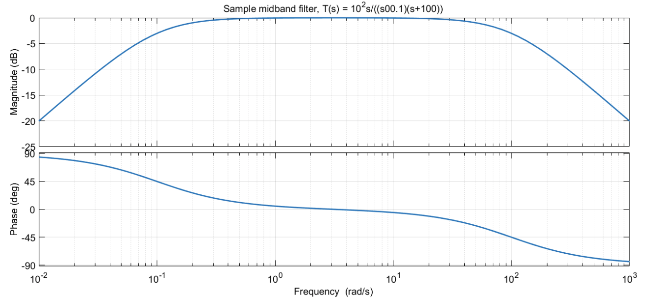
This is all fair and good but it only works if we are working with sine waves.

Most functions are not sine waves… but what if they (i.e. functions we care about) can be written as a linear combination of sine waves?

Fourier series:

Fourier series are obviously useful when working with systems, but they are also useful when working with signals on their own.

We will first work with a classic signal example that was a major problem in the days of the telegraph,

• in the early days of landline phones,
• in the early days of cell phones and the early Internet,
• Is the reason why we developed 5G,
• and will continue to be a problem for the foreseeable future.

”Recall” Taylor’s theorem from MATH119:

Theorem 1: Taylor's Thorem

Let $k\ge 1$ be an integer and let $f$ be a real valued function that is differentiable at least $k$ times at some point $a\in \mathbb{R}$. Then there exists a real valued function $h_k$ such that

and ${\lim }_{x\to a}{h}_k(x)=0$.

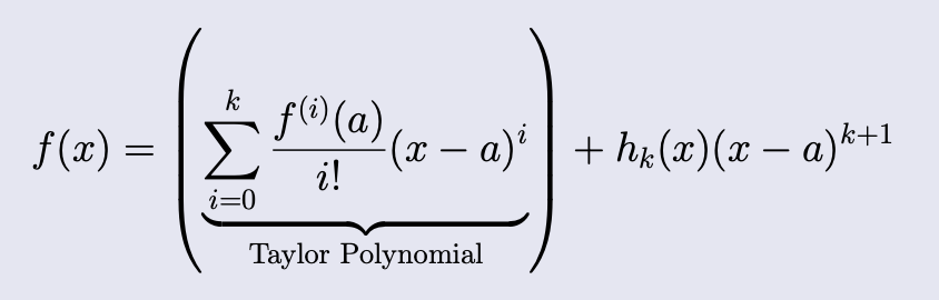
For infinitely differential functions $f$ we can write

$$f(x)=\sum _{i=0}^k\frac{f^{(i)}(a)}{i!}(x-a{)}^i$$

Examples: $e^x=\sum _{i=0}^{\infty }\frac{x^i}{i!}$, or $sin(x)=\sum _{i=0}^{\infty }(-1)\frac{x^{2i+1}}{(2i+1)!}$.

Here we used the basis $\{x^n|n\in \{0,1,2,...\}\}$ but what if…

somehow… $\{sin(nx)|n\in \{0,1,2,3,...\}\}$ could be used as a basis for some set of functions?

This would synchronize well with LTIs and it is what we will study for the rest of this course.

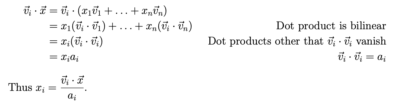
MATH115 orthogonal basis “review” part 2 (see L3 for the version we used for Laplace transforms):

Suppose that there is a orthogonal basis $\{\overrightarrow{v_1},...,\overrightarrow{v_n}\}$ for ${\mathbb{R}}^n$.

This means that $\overrightarrow{v_i}\cdot \overrightarrow{v_j}=a_i\delta [i-j]$ where $a_i\ne 0$.

If we wanted to write $\vec{x}\in {\mathbb{R}}^n$ in this basis we would need to solve the system of equations

$$\vec{x}=x_1\overrightarrow{v_1}+...+x_n\overrightarrow{v_n}.$$

We can solve this using orthogonality (as in L3). Explicitly to find $a_i$ we take the dot product with $\overrightarrow{v_i}$:

To make this method work for $\{sin(nx)|n\in \{0,1,2,3,...\}\}$ we MUST

• Find a “dot product”, called an inner product, for functions such that "$sin(nx).sin(mx)=a_n\delta [n-m]$" and compute the $a_{n}s$.
• Define (the different types of) convergence for series of functions i.e. $f(x)=\sum _{i=0}^{\infty }sin(nx)$.

To fft_fun.m

To voice analyzing phone thing!!

In subsequent lectures we will:

• Generalize the dot product to functions
• Learn how to use this new dot product to compute a few different versions of Fourier series (sin, cos, half sin, half cos and complex exponential),
• Talk about convergence and what the Fourier series for $f(x)$ converges to (it is not always $f(x)!!$) and
• Talk about the Fourier transform (which is just the 2-sided Laplace transform when $s=jw$).

Lecture 21 - $L^2$ space, inner product on $L^2$, and computing Fourier coefficients

Lecture goals:

• know what the standard inner product in $L^2$ is
• and know how to use it to compute Fourier coefficients of $\tau -$periodic functions.

In general properly defining a dot product for functions is a huge issue so we will only work with a special class of functions called “Lebesgue square integrable functions” or L2 functions which makes things nice:

Definition 1: L^{2} functions

A complex valued function $f$ is in the class $L^2([a,b])$ if

${\int }_a^b|f(x){|}^{2}dx$

exists and is finite.

$f$ is in the class $L^2$ if

${\int }_{-\infty }^{\infty }|f(x){|}^{2}dx$

exists and is finite.

$L^2$ and $L^2([a,b])$ form vector spaces so ideas from MATH115 can be used (with proper adjustments). Now if $f$ is a member of $L^2([\frac{-\tau }{2},\frac{\tau }{2}])$ for some fixed $\tau$ then our goal is to write

$$f(t)=\sum _{n=-\infty }^{\infty }{c}_n{e}^{\frac{2\pi n}{\tau }}jt$$

for $t\in [\frac{-\tau }{2},\frac{\tau }{2}]$.

To do this we need to somehow solve for the $c_{n}s...$

By comparison with how we solved

$$\vec{b}=c_1\overrightarrow{v_1}+...+c_n\overrightarrow{v_n}$$

for an orthogonal basis $\{v_1,...,v_n\}$

We need a…

Inner product for L^{2}([-\tau,\tau])

Recall that if $\vec{x},\vec{y}\in {\mathbb{C}}^n$ then

$$\vec{x}\cdot \vec{y}=x_1\overline{y_1}+x_2\overline{y_2}+...+x_n\overline{y_n}$$

Now if $f$ and $g$ are complex valued functions, then the “dot product”, which will be called an inner product, should follow a similar definition,.

The summation becomes integration!!!

Definition 2: Standard Inner product on L^{2}([a,b])

If $f$ and $g$ are complex valued functions in $L^2([a,b])$ then the standard inner product is

$⟨f,g⟩=\frac{1}{b-a}{\int }_a^{b}f(t)\overline{g(t)}dt$

Theorem 1: Existence of Inner Product

If $f,g\in L^2([a,b])$ then $⟨f,g⟩$ exists and is finite.

We skip the proof since it needs some real analysis…

Theorem 2

The set of complex exponentials $\{e^{\frac{2\pi n}{\tau }jt}|n\in \{0,\pm 1,\pm 2,...\}\}$ is an orthonormal basis for a subspace of $L^2([\frac{-\tau }{2},\frac{\tau }{2}])$.

Partial proof: We will not prove that the collection is linearly independent but will prove that they are orthonormal.

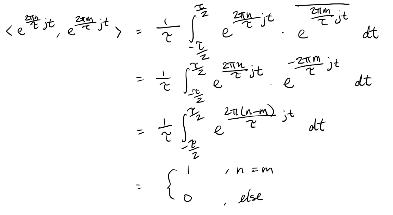
Now that we have an orthonormal basis for a subset of $L^2([\frac{-\tau }{2},\frac{\tau }{2}])$, we can project any function in $L^2(\frac{-\tau }{2},\tau )$ into our basis $\{e^{\frac{2\pi n}{\tau }jt}|n\in \{0,\pm 1,\pm 2,...\}\}$ by using our inner product.

Note that since we are doing a projection and the basis may not be (is not…) a basis for $L^2([\frac{-\tau }{2},\frac{\tau }{2}])$, the result of projecting into this basis may not be equal to the original function in the traditional sense.

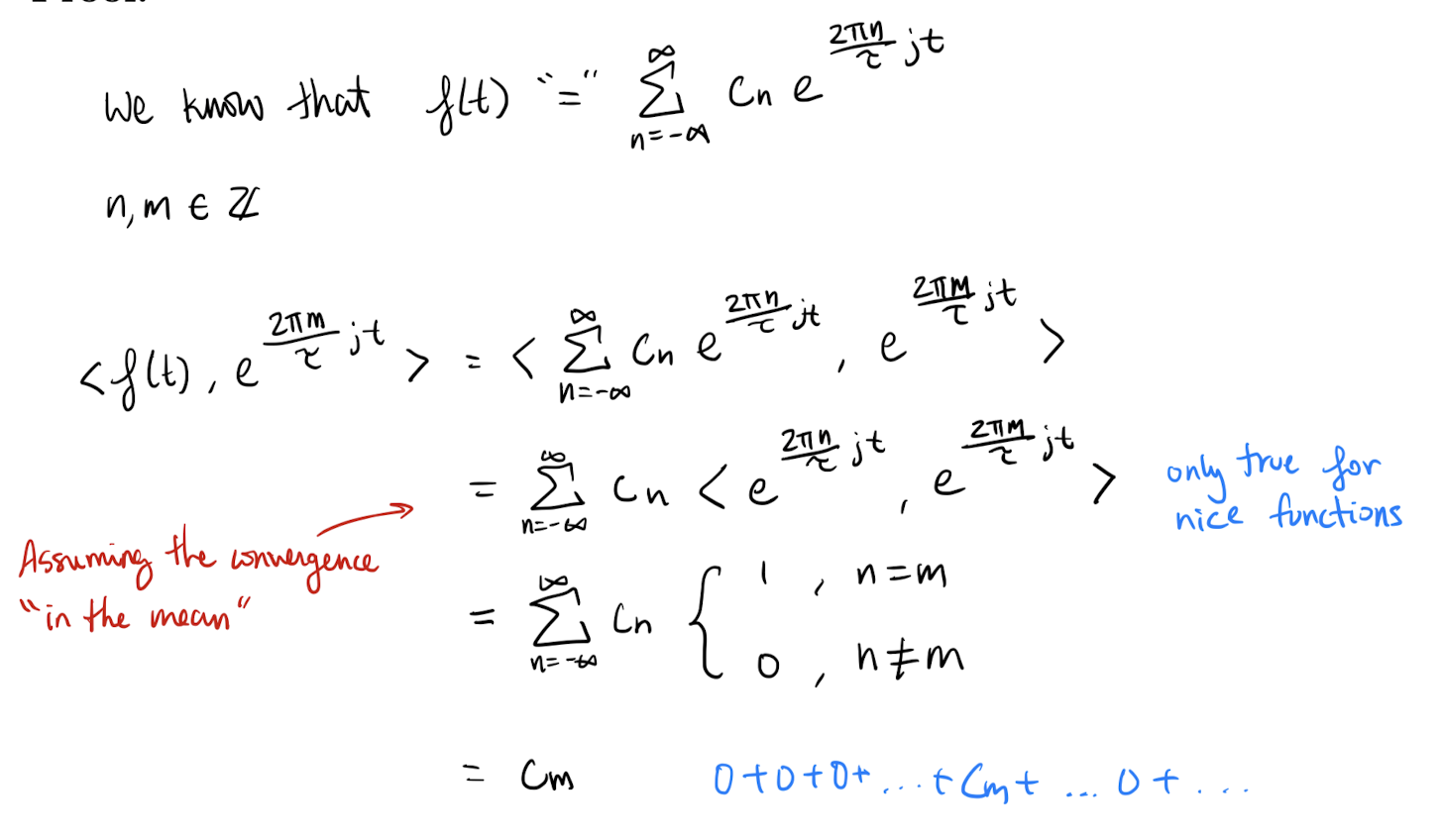
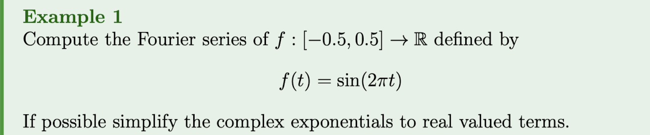
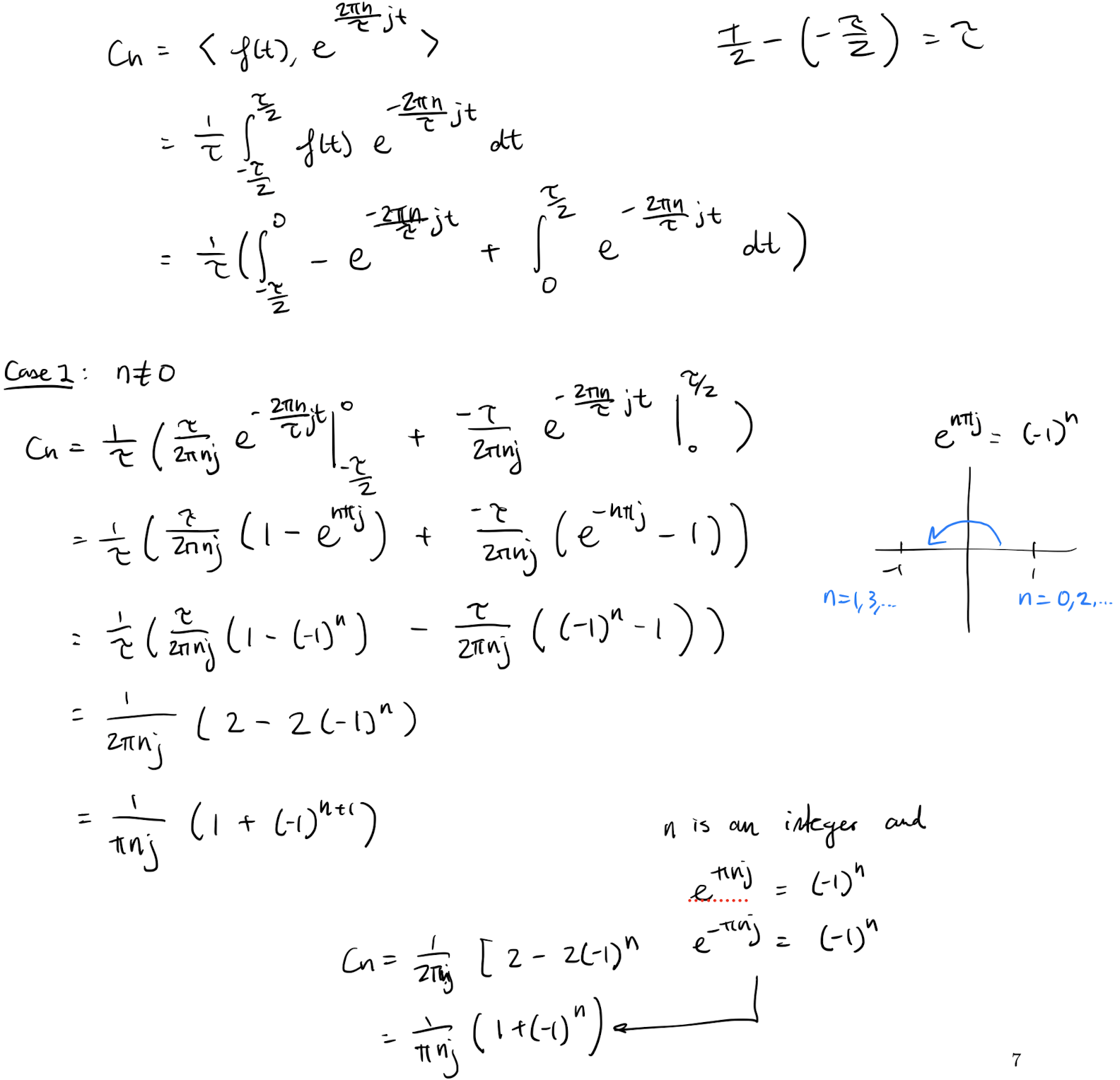
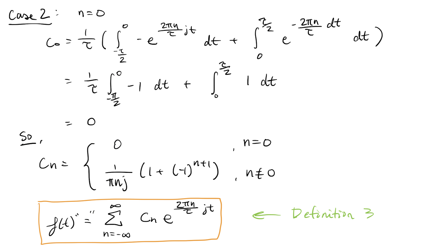
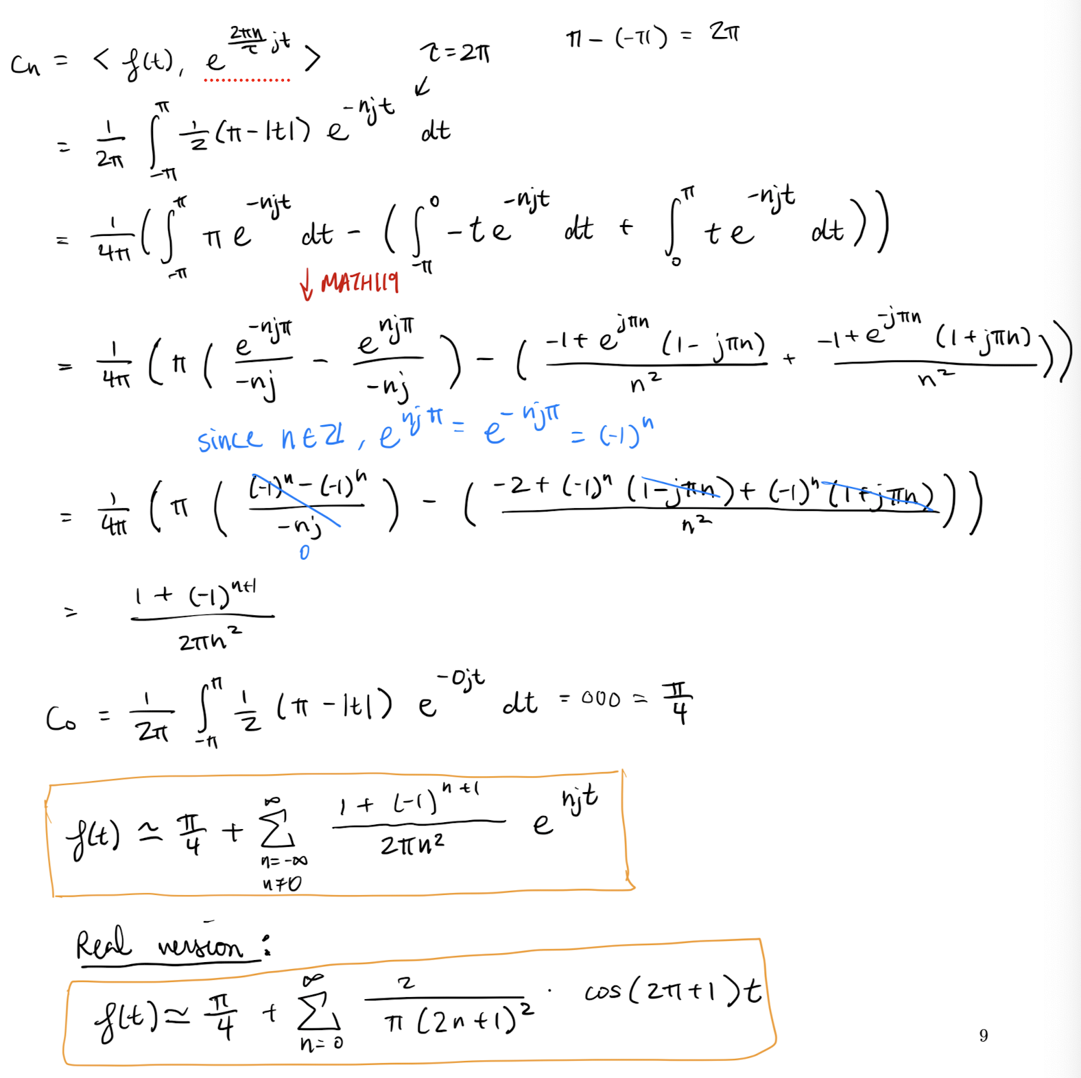
Definition 3: Fourier Series - Complex Form

If $f\in L^2([\frac{-\tau }{2},\frac{\tau }{2}])$ then the Fourier series in complex form of $f(t)$ is

$\sum _{n=-\infty }^{\infty }{c}_n{e}^{\frac{2\pi n}{\tau }jt}$

where the $c_n$ are found by projecting $f$ into the basis of complex exponentials.

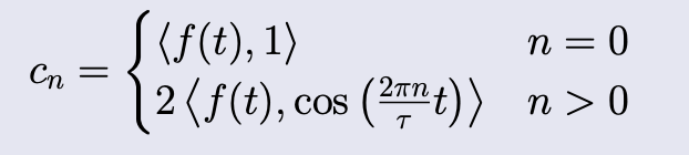
Theorem 3: Fourier Coefficients for Series in Complex Form

If $f\in L^2([\frac{-\tau }{2},\frac{\tau }{2}])$ then the Fourier coefficients $c_n$ of $f(t)$ are

$c_n=⟨f(t),e^{\frac{2\pi n}{\tau }jt}⟩$.

If $f$ is real valued than $c_n=\overline{c_{-n}}$.

Proof:

Compute the things!!!

Where does the C_{n} values come from??? And the options...?

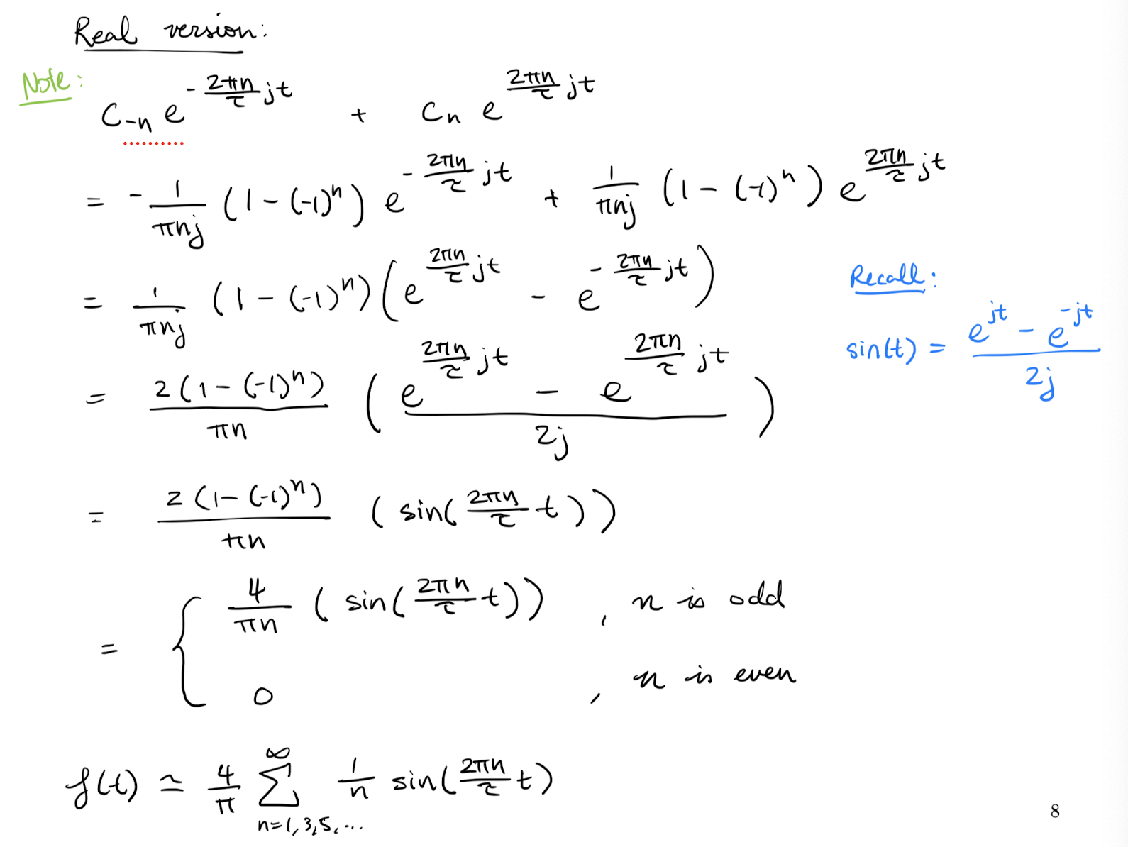
What is the purpose of the Real version???

Lecture 22: Real Fourier series and convergence

Lecture goals:

• Know how to find the real Fourier series quickly and
• know the convergence properties of Fourier series.

$\tau$ periodic functions:

Definition 1: \tau periodic functions

A $f$ function defined on $\mathbb{R}$ is $\tau$ periodic if for all $t\in \mathbb{R}$

$f(t)=f(t+\tau )$.

Generally, we pick the smallest value of $\tau$ such that the above holds.

Theorem 3 ($L^2$) from L21 holds for $\tau$ periodic functions and we would integrate over one period.

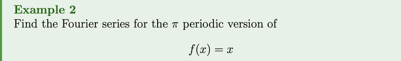
If I ask you to find the Fourier series without telling you a domain for f and f is \tau periodic,

then you first find out the $\tau$ period of $f$ and do the computation over a period of $f$.

Fourier sin/cos series:

For a real valued function sometimes we found the Fourier Series simplified to a sum of sine waves and sometimes it resulted in a sum of cos waves. We now elaborate on this:

Definition 2: Even and odd functions

A function $f$ is even if

$f(-t)=f(t)$

A function $f$ is odd

$f(-t)=-f(t)$

$\forall t\in \mathbb{R}$.

Theorem 1

For a real valued, $\tau$ periodic function $f\in L^2([\frac{-\tau }{2},\frac{\tau }{2}])$:

• If $f$ is an even then the Fourier series can be simplified to a sum of cos waves.
• If $f$ is an odd then the Fourier series can be simplified to a sum of sin waves.

The sums above are called Fourier cosine series and Fourier sine series respectively.

For completion we will write Theorem 3 from L21 for sin and cos series.

Theorem 2: Fourier Sine and Cosine Coefficients

If $f$ is a real valued function that is in $L^2([\frac{-\tau }{2},\frac{\tau }{2}])$ then

• If $f$ is even then the Fourier cosine series for $f$ is

$\sum _{n=0}^{\infty }\cos (\frac{2\pi n}{\tau }t)$

where

• If $f$ is odd then the Fourier sine series for $f$ is

$\sum _{n=1}^{\infty }{s}_n\sin (\frac{2\pi n}{\tau }t)$

where

$s_n=2⟨f(t),(\frac{2\pi n}{\tau }t)⟩$

Sketch of proof:

• Start with the coefficients in Theorem 3,
• write the complex exponential in terms of sin/cos waves,
• simplify the integrals by using the properties that
  • the integral of an odd function over $[-a,a]$ for any $a\in \mathbb{R}$ is 0,
  • that $g(-x)+g(x)=0$ for an odd function $g$ and
  • that $g(-x)+g(x)=2g(x)$ for an even function $g$.

I strongly suggest not blindly memorizing this but to instead memorize Theorem 3 and then understand how it still simplify if there are no sin or cos terms.

This is similar to the computations seen in the last lecture

Theorem 3

If $f$ is real then we can decompose it into even and odd functions as follows:

$f_{even}(t)=\frac{f(t)+f(-t)}{2}$

and

$f_{odd}(t)=\frac{f(t)-f(-t)}{2}$

$f(t)=f_{even}(t)+f_{odd}(t)$.

Sketch of proof: Show that $f_{even}$ is even, that $f_{odd}$ and that when summed we get $f$.

Theorem 4

Every real valued function in $L^2([\frac{-\tau }{2},\frac{\tau }{2}])$ admits a real valued Fourier series with some sin and/or cos terms. i.e. the complex form will always simplify to sin and cos terms.

Sketch of proof: Since $f$ is real, it can be decomposed into an even and odd part. The even part gives us a cos series and the off part gives us a sin series.

Need to know how to integrate sin and cos...

It is Integration By Parts…

What is s_{n}?

In theorem 3. In this example, somehow $\tau =\pi$. We find $s_n$ in order to solve the problem $f(x)$.

https://piazza.com/class/lr4fiutz6vg69z/post/441

In the prof’s notes, he did $c_n$ for $x^2+1$.

Types of Convergence:

In MATH119 you dealt with the convergence of series of real numbers. Things like

$$\sum _{i=1}^{\infty }0.9^i$$

In these cases there is a natural way to define convergence (though this is not actually unique).

With sums of functions like this

$$\sum _{i=0}^{\infty }{f}_i(x),$$

there are many different ways to define convergence:

Definition 3: Some Types of Convergence

If $f_1,f_2,...,f_n$ is a sequence of $L^2$ functions defined on $[a,b]$ then we say that

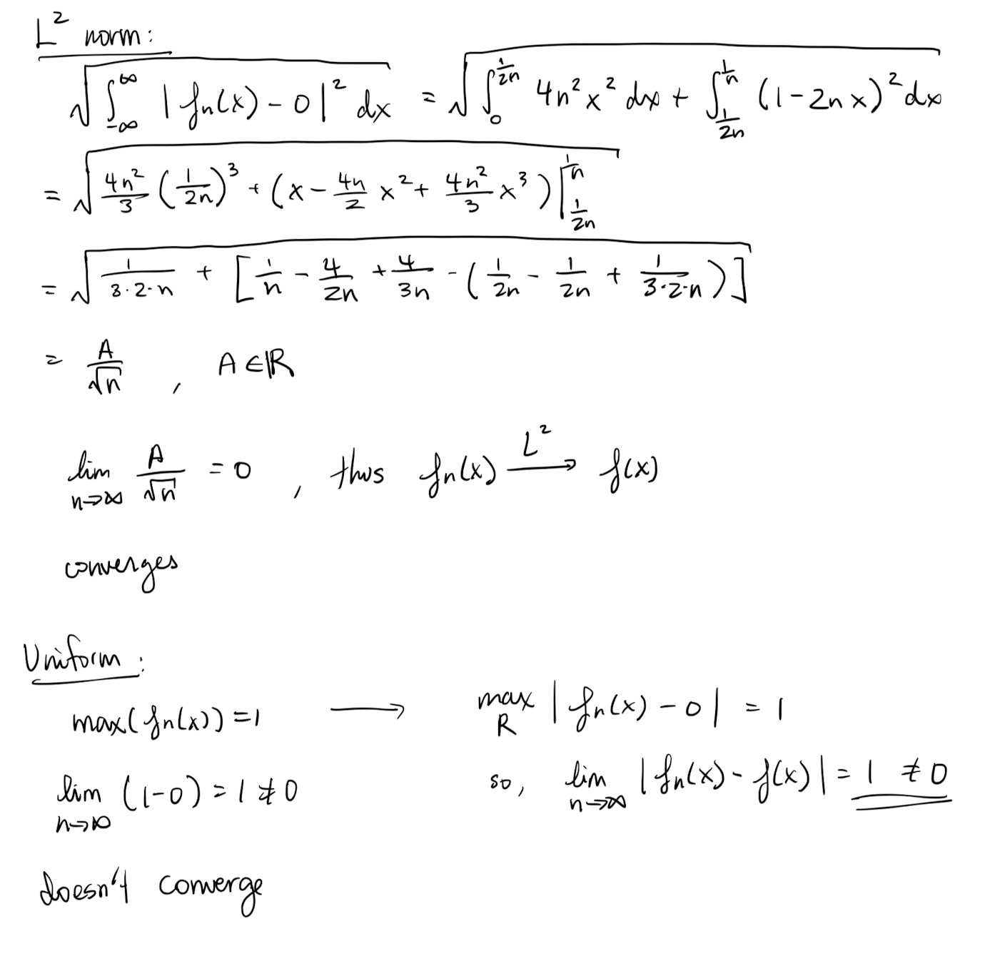
• the sequence converges in the $L^2([a,b])$ norm, or converges in the mean or converges almost everywhere, to $f$ is

${\lim }_{n\to \infty }\sqrt{{\int }_a^b|f_n(x)-f(x){|}^{2}dx}=0$

tldr; the “average error” goes to 0.

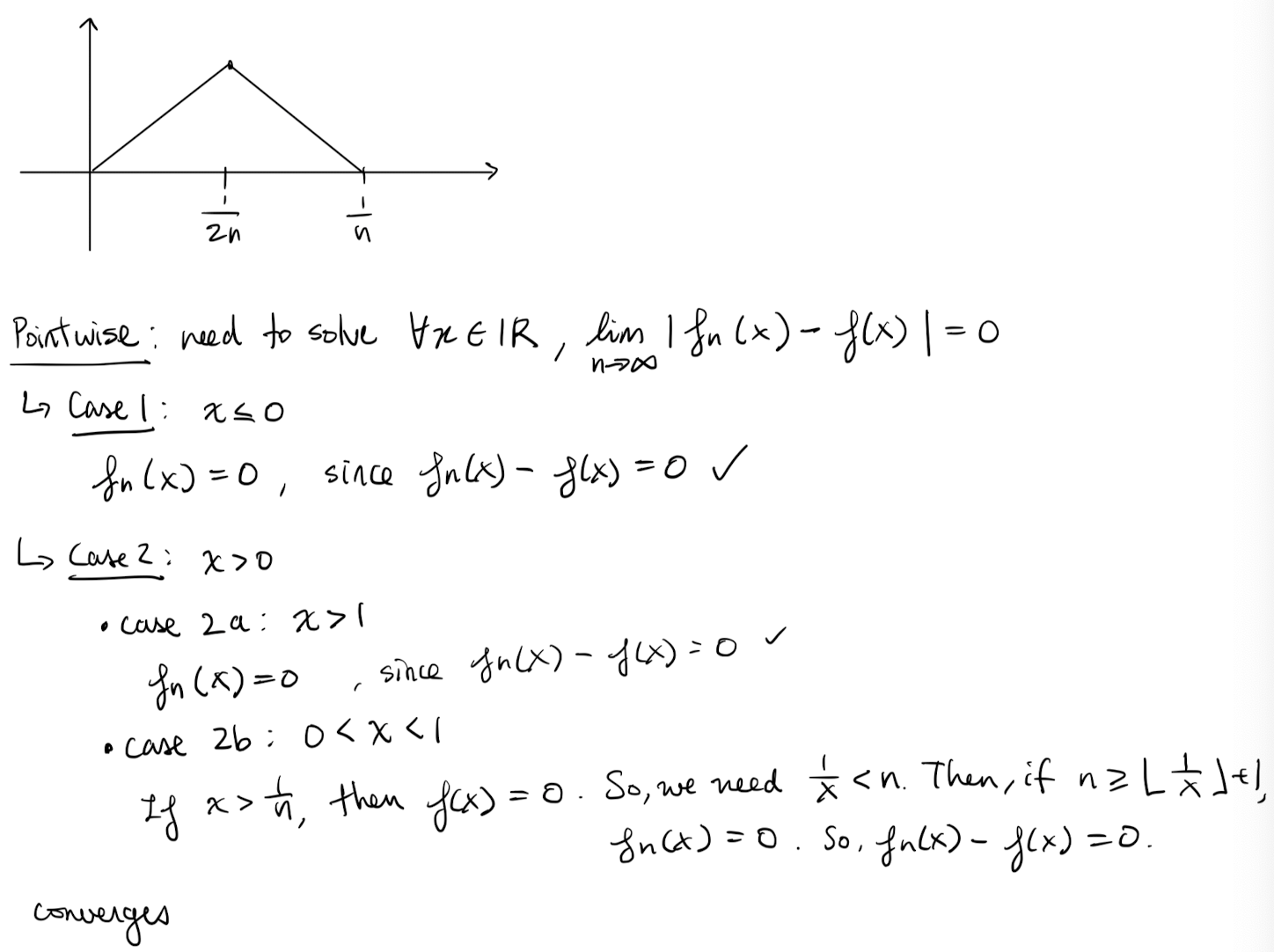
• the sequence pointwise converges to $f$, if for any $x\in [a,b]$

${\lim }_{n\to \infty }(f_n(x)-f(x))=0$

tldr; the error at each point goes to 0.

• The sequence uniformly converges to $f$ if

${\lim }_{n\to \infty }{\max }_{[a,b]}|f_n(x)-f(x)|=0$

If the maximum does not exist then we replace it with the smallest upper bound (called the sup).

tldr; the maximum error converges to 0.

Note that each of the things we take the limit of are just numbers!
Metanote, the first bullet point can be called by all those names only when we talk about functions on a finite interval (that is the case for this course).

• https://piazza.com/class/lr4fiutz6vg69z/post/467
• • https://piazza.com/class/lr4fiutz6vg69z/post/443: Reasoning for these two cases $x\le 0$, $x>0$.

Convergence of Fourier series:

Before talking about the convergence of Fourier series, we need to introduce some new definitions.

Definition 4: Piecewise C^{1}

A function $f$ is a Piecewise $C^1$ (PWC1) on the interval $[a,b]$ if there is a finite partition $a=t_0<t_1<...<t_k=b$ such that:

• $f^{\prime }$ exists on each interval $(t_i,t_{i+1})$,
• $f^{\prime }$ is continuous on each interval $(t_i,t_{i+1})$,
• $f$ and $f^{\prime }$ are bounded on each interval $(t_i,t_{i+1})$.

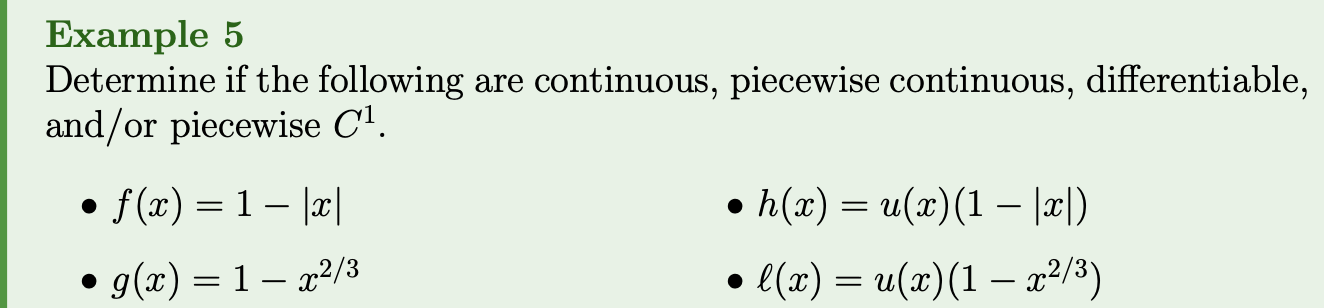
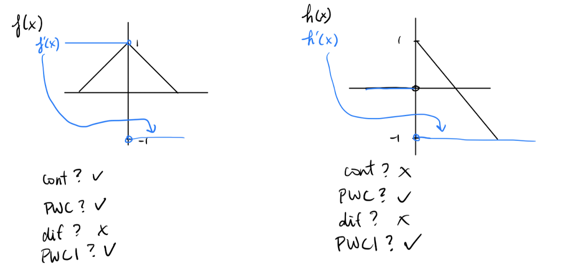
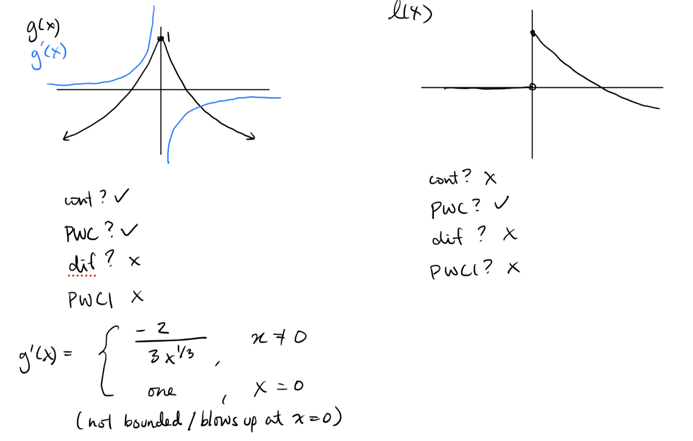
How to determine a function is differentiable and why f(x) and h(x) in the examples are not differentiable?

https://piazza.com/class/lr4fiutz6vg69z/post/478

Differentiable = has a derivative. To see why, ask yourself what the slope is at $x=0$.

1. $f(x)=1-|x|$

• This function is continuous everywhere except at $x=0$, where there’s a sharp corner due to the absolute value function.

2. $g(x)=1-x^{\frac{2}{3}}$

• This function is continuous everywhere, including at $x=0$, since the root is defined for negative values of $x$.

3. $h(x)=u(x)(1-|x|)$

• Here, $u(x)$ is the unit step function, which equals 1 for $x\ge 0$ and 0 for $x<0$.
• Similar to $f(x)$, $h(x)$ is continuous everywhere except at $x=0$, where it has a sharp corner due to the absolute value function.

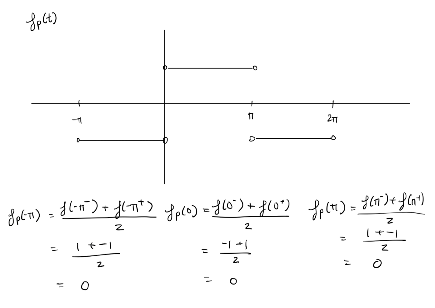
Definition 5: Periodic Extension

The periodic extension of a function $f$ defined on $[a,b]$ is the $b-a$ periodic function $f_p$ such that

• $f_p(t)=f(t)$ for $t\in (a,b)$ where $f(t)$ is continuous.
• $f_p(t)=\frac{f(t^{-})+f(t^{+})}{2}$ for $t\in (a,b)$ where $f(t)$ is not continuous
• $f_p(a)=\frac{f(a)+f(b)}{2}=f_p(b)$

Theorem 5: Convergence of Fourier series

Let $f_p$ be the periodic extension of a function $f\in L^2([\frac{-\tau }{2,\frac{}{\tau }}2])$.

• The Fourier series of $f$ converges in the $L^2$ norm (also in the mean and almost everywhere) to $f$ (and also $f_p$) on any finite subinterval of $[\frac{-\tau }{2},\frac{\tau }{2}]$.
• If $f_p$ is piecewise $C^1$ then the Fourier series of $f$ converges pointwise to $f_p$ for all $x\in \mathbb{R}$
• If $f_p$ is piecewise $C^1$ and continuous then the Fourier series of $f$ converges uniformly $f_p$ on any finite interval of $\mathbb{R}$.

The proof is beyond the scope of this course.

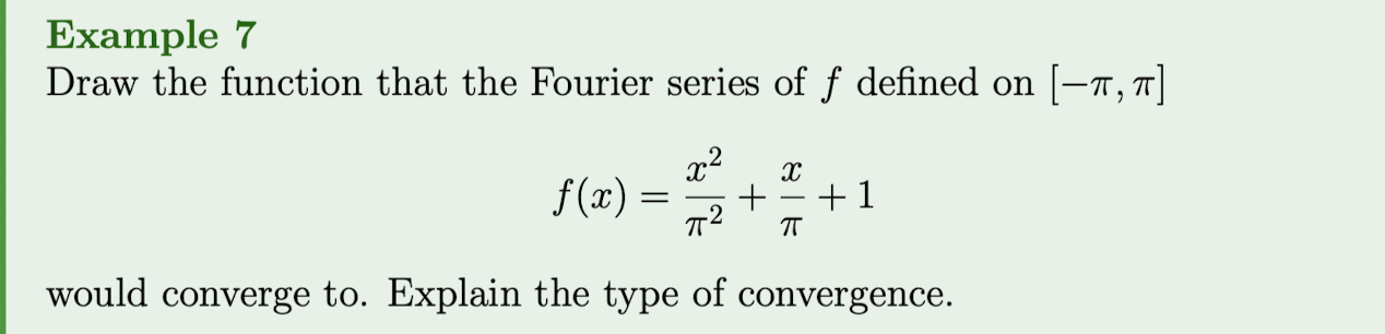
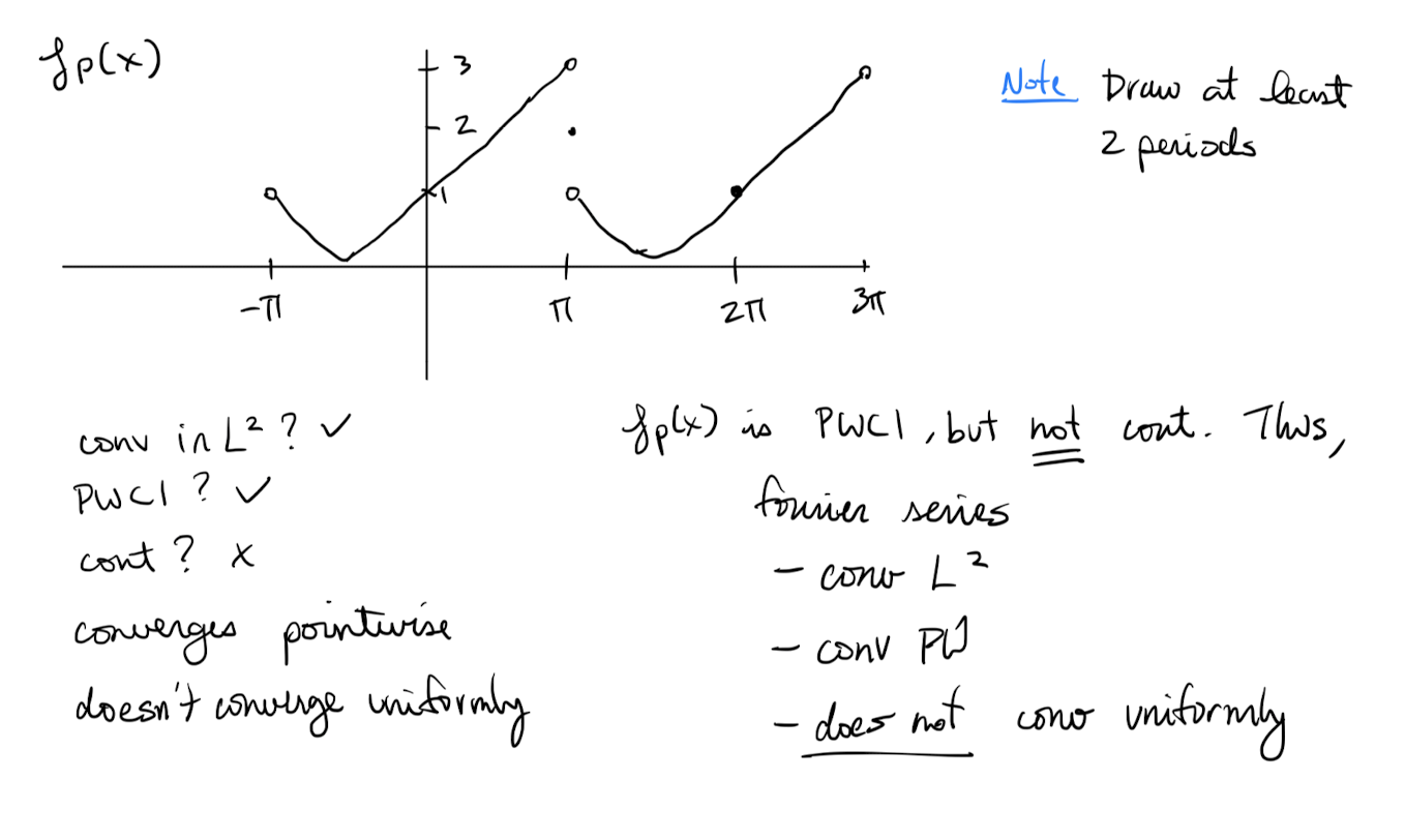
Are we supposed to know how to graph this????

By heart?

Why is it PWC1? and not continuous?

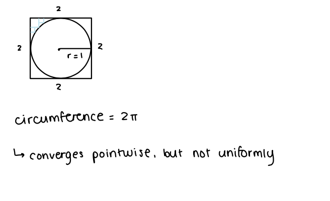
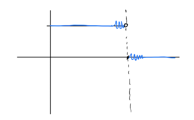
Definition 6: Gibbs Phenomenon

For a $L^2([a,b])$ function $f$ with periodic extension $f_p$, if $f_p$ is not continuous at some point $t_0$ then truncated Fourier series of $f$ will have growing oscillations near the point $t_0$. This is called Gibbs Phenomenon.

These oscillations do not appear in the infinite sum.

Gibbs Phenomenon is a characteristic behaviour observed in truncated Fourier series when dealing with functions that have discontinuities. Here's a breakdown of the definition:

1. Function with Periodic Extension: Consider a function $f$ defined on an interval $[a,b]$ with a periodic extension $f_p$​ that repeats the function periodically outside this interval.
2. Discontinuity at​ $t_0$: If the periodic extension $f_p$​ of ff is not continuous at some point t0t0​ within its period, then we have a discontinuity at $t_0$​.
3. Truncated Fourier Series: When we approximate ff using a truncated Fourier series, we’re essentially using a finite sum of Fourier coefficients to approximate the function. This finite sum doesn’t capture all the frequency components of the original function.
4. Growth of Oscillations: Near the point $t_0$​ where the periodic extension $f_p$​ is discontinuous, the truncated Fourier series will exhibit oscillations that grow as we approach $t_0$​.
5. Gibbs Phenomenon: This growth of oscillations near discontinuities in the periodic extension is known as Gibbs Phenomenon.
6. Absence in the Infinite Sum: Interestingly, despite these growing oscillations in the truncated series, they do not appear in the infinite sum of the Fourier series. The infinite sum captures all the frequency components of the original function and thus provides a smoother approximation.

Lecture 23: Differentiating and integrating Fourier series, Persivalle and Dirichlet theorems and Fourier transform

Lecture goals:

• Know when you can term-wise integrate and differentiate Fourier series,
• what the Persivalle and Dirichlet theorems state
• and how to use Persivalle’s theorem.

Integrating and differentiating Fourier series:

For general series of piecewise convergent functions

$$f(x)=\sum _{n=-\infty }^{\infty }{f}_n(x)$$

it is NOT true that

$$f^{\prime }(x)=\sum _{n=-\infty }^{\infty }{f}_n^{\prime }(x)$$

or that

$$\int f(x)dx=\sum _{n=-\infty }^{\infty }\int f_n(x)dx.$$

So when can we do this for Fourier series?

Theorem 1: Term-by-term integration of Fourier series

The Fourier series of a PWC1 $\tau -$periodic $L^2$ function $f(t)$ can be term-by-term integrated to give a convergent series that pointwise converges (and sometimes uniformly) over any finite interval.

tldr; If PWC1, integral has uniform convergence. Else, pointwise convergence.

Explicitly if $f_p$ is in $L^2$ and $f_p(t)=\sum _{n=-\infty }^{\infty }{c}_n{e}^{\frac{2\pi njt}{\tau }}$

then ${\int }_a^b{f}_p(t)dt=\sum _a^t{e}^{\frac{2\pi njt}{\tau }}dt$

and the convergence is at least pointwise.

Note 1: It is because of this theorem, that we can guarantee the existence of the Fourier coefficients derived in L21.

Note 2: If the Fourier series has a non-trivial constant $a_0$ term then when integrated we obtain $a_{0}t$ which means that the RHS might not be a Fourier series.

Theorem 2: Term-by-term differentiation of Fourier series

Let $f$

• be a PWC1 $\tau -$periodic function,
• be a continuous function and
• satisfy $f(\frac{-\tau }{2})=f(\frac{\tau }{2})$

If the above conditions are met then the series for $f$ can be term-by-term differentiated to give a pointwise convergent series that pointwise converges to $f_p^{\prime }(t)$ on for all $t$ such that $f_p^{\prime \prime }(t)$ exists

Explicitly if $f$ satisfied the above and $f_p(t)=\sum _{n=-\infty }^{\infty }{c}_n{e}^{\frac{2\pi njt}{\tau }}$

then $f_p^{\prime }(t)=\sum _{n=-\infty }^{\infty }{c}_n\frac{d}{dt}{e}^{\frac{2\pi njt}{\tau }}$

and the convergence is pointwise for all points where $f_p^{\prime \prime }(t)$ exists.

f these conditions are met,

then the series for $f$ can be differentiated term-by-term. This yields a pointwise convergent series that converges pointwise to $f_p^{\prime }(t)$ for all $t$ where $f_p^{\prime }(t)$ exists.

In other words, if $f_p(t)$ is the ττ-periodic extension of $f(t)$ satisfying the given conditions, then we can differentiate its Fourier series term-by-term. The resulting series converges pointwise to $f_p^{\prime }(t)$ wherever $f_p^{\prime }(t)$ exists.

• https://piazza.com/class/lr4fiutz6vg69z/post/446

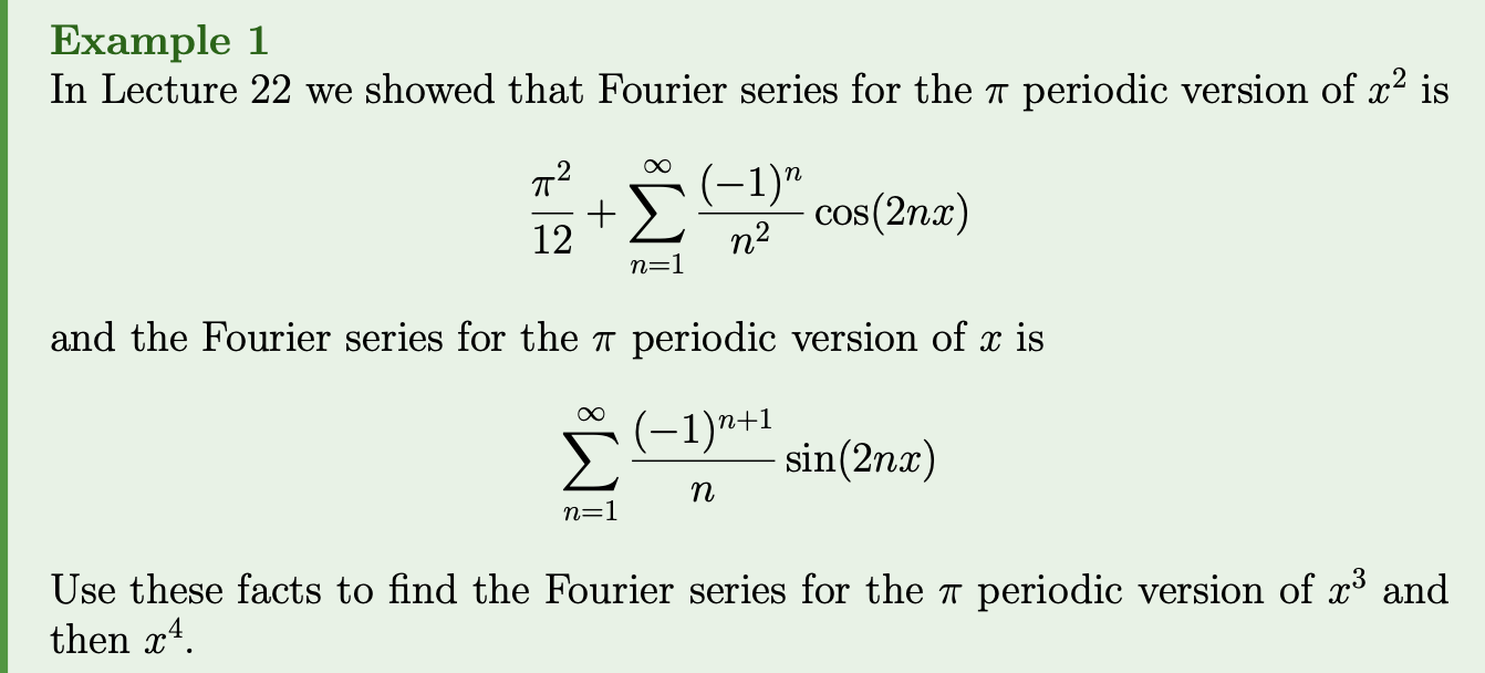
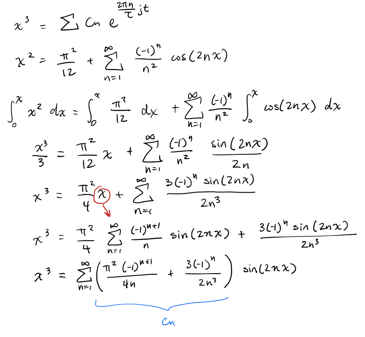
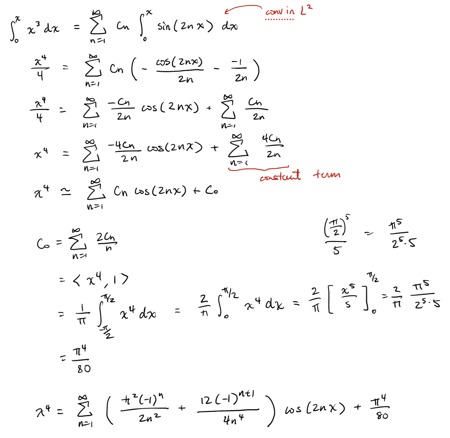
Recall that (although I did not previously name it in L22 Theorem 5):

Theorem 3: Dirichlet's theorem

If $f$ is PWC1 and $\tau$ periodic then the Fourier series of $f(t)$ converges pointwise to $f_p(t)$.

If we define the error of a truncated Fourier series to be

$$e_N(t)=f_p(t)-\sum _{n=-N}^N{c}_n{e}^{\frac{2\pi njt}{\tau }}$$

Then the above theorem tells us that for PWC1 $\tau$ periodic functions $f$,

$$\underset{N\to \infty }{\lim }⟨e_N,e_N⟩=0$$

i.e. the average error goes to zero in the limit. In other words:

Theorem 4: Parseval's theorem

If $f$ is $L^2[\frac{-\tau }{2},\frac{\tau }{2}]$ and $\tau$ periodic function then

$\frac{1}{\tau }{\int }_{\frac{-\tau }{2}}^{\frac{\tau }{2}}|f(t){|}^{2}dt=\sum _{n=-\infty }^{\infty }|c_n{|}^2$

The term $\frac{1}{\tau }{\int }_{\frac{-\tau }{2}}^{\frac{\tau }{2}}|f(t){|}^{2}dt$ is the average energy of wave and hence

• this gives us a way to compute the energy of a wave from the Fourier coefficients (i.e. using fft)
• to determine how many terms we need to include in a truncation of the Fourier series to approximate the original signal to some given power,
• or to derive many useful formulas for computing sums…

Before giving an example, here is the real valued version of Parseval’s theorem:

Theorem 5: Parseval's theorem

If $f$ is a real valued PWC1 and $\tau$ periodic function then $\frac{1}{\tau }{\int }_{\frac{-\tau }{2}}^{\frac{\tau }{2}}|f(t){|}^{2}dt=c_0^2+\frac{1}{2}\sum _{n=1}^{\infty }(c_n^2+s_n^2)$

where $c_n$ and $s_n$ are the Fourier sine and cosine coefficients.

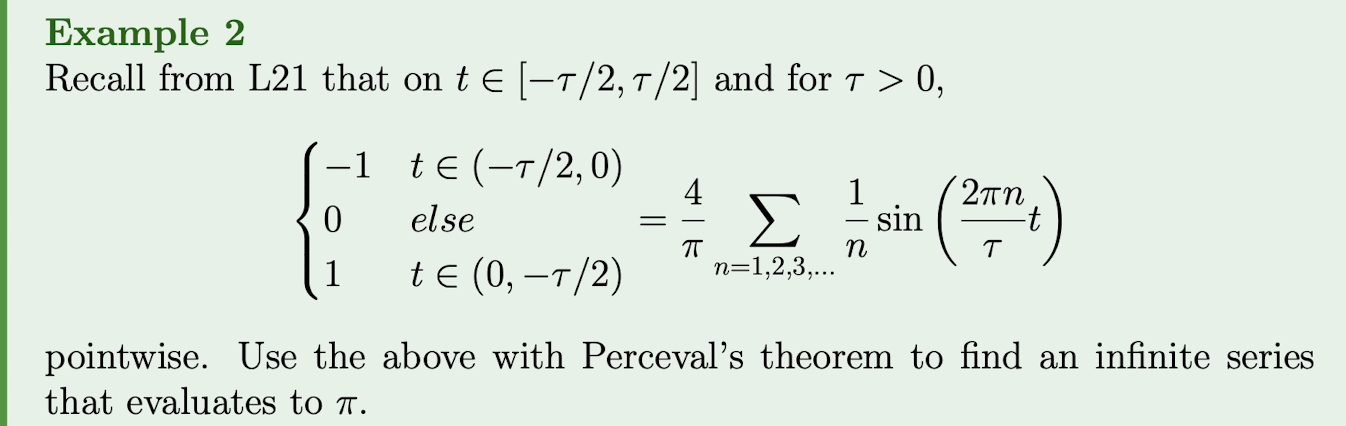
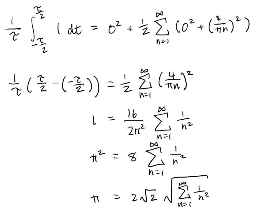
Fourier transform (tldr;):

Recall that the two sided Laplace transform was defined by

$$\mathcal{L}\{f(t)\}={\int }_{-\infty }^{\infty }f(t)e^{-st}dt$$

given that the integral converged.

When working with (causal) DEs, we used the one sided version of the above.

In our work with Fourier series, we required that the functions be $\tau$ periodic. If this is not the case, then our methods do not work!!

What do we do with these cases? Recall

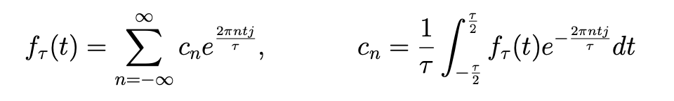
If $\tau \to \infty$ then $n$ is not allowed to be continuous so $c_n$ becomes a function of $\mathbb{R}$ and the discrete sum becomes an integral. Further we would need to do some regularization to deal with the averaging in $c_n$. Doing this defining $w$ to be the limiting values of $\frac{2\pi n}{\tau }$ (and some complex analysis to deal with the regularization) gives:

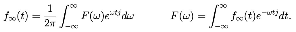
$F(w)$ is called the Fourier transform of $f_{\infty }$ and we write $F(w)=F\{f_{\infty }\}$ explicitly:

Definition 1: Fourier Transform

If $f\in L^1$ then the Fourier transform of $f$ is

$F(w)=F\{f(t)\}={\int }_{-\infty }^{\infty }f(t)e^{-wtj}dt$

and the inverse Fourier transform of $F(w)$ is

$f(t)=F\{F(w)\}=\frac{1}{2\pi }{\int }_{-\infty }^{\infty }F(w)e^{wtj}dw$

Note that the Fourier transform/inverse transform is just the two-sided Laplace transform in the case that $s=wj$.

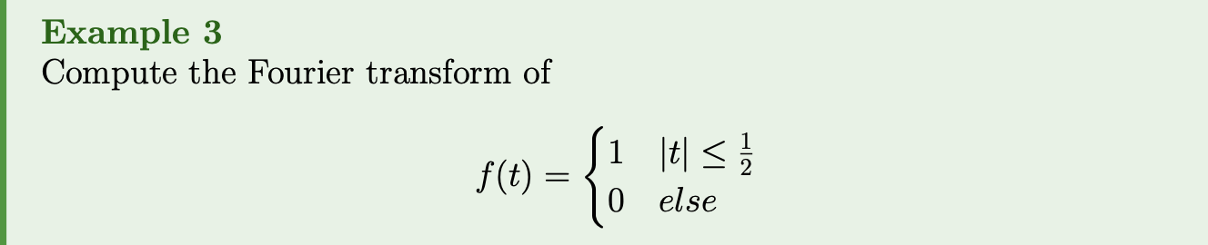
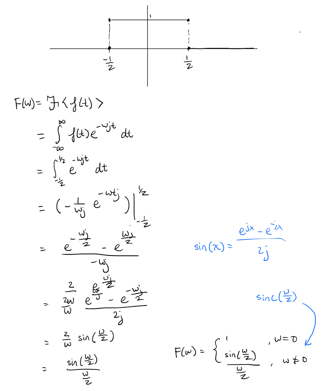
The End.