Labs ECE358

Lab 1

Delay and packet loss are two performance metrics of computer networks

Delay:

Measure of the time it takes the packet to reach from its source to its destination.
Queueing delay: delay that is incurred while the packet is waiting its turn in the queue to be processed

Packet loss

Percentage of data packets that are lost in the system
Happens when a packet is received in a finite queue that is already full. So the queue does not have enough buffer to store the packet and the packets has to be dropped.

We try to get an approximate analytical model which is validated with a simulation model.

4.1 Kendall Notation

Queues are typically described using Kendall notation of the form: A/S/C/K/D, where

A corresponds to the arrival process of the packets (more precisely the distribution of the inter-arrival time between packets). A can be M (Markovian), D (Deterministic) or G (General).
S corresponds to the server process for the packets. S can again be M, D or G.
C corresponds to the number of servers (or network interfaces).
K corresponds to the buffer size, i.e. the number of packets that can be accommodated in the “waiting room”. If omitted, the buffer is assumed to be infinitely large.
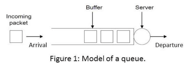
D corresponds to the queueing discipline, which is almost always FIFO (First-In-First-Out) see Figure 1. and is therefore often omitted from the notation.

For example, M/M/c queue means that both the arrival and service processes are Markovian and that there are c servers. For the purposes of this lab, a Markovian arrival process means that the arrival process follows a Poisson distribution. In a Poisson distribution, the distribution of the time between successive arrivals (also called inter-arrival time) is modeled via an exponential distribution. A service process M means that the distribution of the service time is identical for each customer/packet, is independent from one customer to another, and is exponentially distributed

The queues you need to simulate in this experiment are M/M/1 and M/M/1/K. We will not be modeling multi-server queues here.

4.2 M/M/1 and M/M/1/K queues

Consider an M/M/1 queue with arrival rate of 10 packets/sec and service rate of 500 packets/sec. In this queue, packets will arrive to the queue following a Poisson process where the queue is expected to receive 10 packets/sec on average. When a packet arrives to the queue, it can be serviced (i.e., transmitted by the server) right away if the queue is empty. If the queue is not empty, an arriving packet has to wait in the queue for its turn to be serviced. Note that the queue size in M/M/1 queue is infinite, and hence, any arriving packet will find a room in the queue and no packet will be dropped. The packet waiting time in the queue (queuing delay) is an important metric to measure the performance of a computer network. In this project, you will measure the queueing delay in different queue models. Once a packet arrives at the server, it will be transmitted with a service rate following an exponential distribution. The service rate of the server depends on the length of each packet, which is assumed to be different for every packet, and the transmission/processing speed of the server. Packets that are longer will take longer to process than packets that are smaller, for the same server speed.

Now let us consider M/M/1/K queue model. The only difference between M/M/1 queue and M/M/1/K is that the buffer size (K) in M/M/1 is infinite while it is limited in M/M/1/K to a size of K packets. As a result, if a packet arrives in an M/M/1/K queue and this queue has already K packets in it, the packet is dropped, i.e., the packet will be lost. Packet loss ratio is another performance metric of a computer network. It is the ratio of packets that are lost to the total number of packets that are received. In this project, you will calculate the packet loss ratio for M/M/1/K queue.

4.2 Basics of Simulation Modeling

A simulation model consists of three kinds of elements: Input variables, Simulator, and Output variables. The simulator is a mathematical/logical relationship between the input and the output. A simulation experiment is simply a generation of several instances of input variables, according to their distributions, and of the corresponding output variables from the simulator. We then use the output variables (usually some statistics) to analyze the performance measures of the system. The generation of the input variables and the design of the simulator will be discussed next.

4.4 Generation of input variables with different distributions

In this project, you will need to simulate random variables with exponential probability distributions. However, common libraries for generating random numbers generate only uniformly distributed variables. Because it is instructive to do so, we will write a short function to generate an exponentially distributed variable from a uniformly generated one using a method called the inverse method.

Presume that our desired distribution is given by F(x), and we can only generate a variable, U, which is drawn from a uniform distribution. In fact, we do not want F(x) (we already know this – it’s the exponential distribution). We want X itself – that is, a variable drawn from the exponential distribution. If you need to generate a random variable X with a distribution function 𝐹(𝑥) using the inverse method, you start by setting

$U = F (x)$ , where $U$ is our uniform random variable in the range (0, 1)

Then find the inverse of the distribution function, i.e.,

x = F^{- 1} (U)

Now, if you generate uniform random variable U in the range (0, 1) and substituted in the previous equation, you will get a random variable 𝑥 that is drawn from a distribution 𝐹(𝑥). You will need to use the inverse method to generate the required random variables for M/M/1 and M/M/1/K.

4.4.1 Generating exponential random variables

Assume that we want to generate an exponential random variable 𝑥 with average $\frac{1}{λ}$ , where $λ$ is the rate parameter. We will use the inverse method. We start by the exponential cumulative distribution function given as:

F (x) = 1 - e^{λ x} (1)

Set $F (x)$ equal to $U$ which is a uniform random variable

F (x) = U (2)

Then, substitute from (1) in (2) and solve for $x$

1 - e^{- λ x} = U e^{- λ x} = 1 - U - λ x = l n (1 - U) x = - \frac{1}{λ} l n (1 - U)

where $U$ is a uniformly generated number and $x$ is the exponential random variable.

4.5 Designing a Discrete Event Simulator (DES)

Discrete Event Simulation (DES) is commonly used to study the performance of evolving systems whose states change at discrete points in time in response to external and internal events. A DES simulator consists of a set of time-ordered events $E i, i = 1, \dots, N$ , along with their occurrences time, such that $t (E i) < t (E i + 1)$ for all $i$ as shown in Table 1. The time of the last event, which is $t (E_{i + 3})$ in this case, is the called the simulation time. Note that there is a difference between the simulation time and the execution time of your code. The execution time is how long your code will run for in order to simulate a system for an amount of time equal to the simulation time.

Table 1. Discrete Event Simulation (DES)

Event	Time
$E_{i}$	$t (E_{i})$
$E_{i + 1}$	$t (E_{i + 1})$
$E_{i + 2}$	$t (E_{i + 2})$
$E_{i + 3}$	$t (E_{i + 3})$

To perform DES, you need to create events and their corresponding occurrence time. But when should the DES terminate? By performing DES, we are performing a statistical experiment. In order to get good results in a statistical experiment, your simulation time should be large enough to truly represent the system under consideration, which is a queue in this case.

An easy way to get stable simulation results is to run the experiment for T seconds, take the result, run the experiment again for 2T seconds and see if the expected values of the output variables are similar to the output from the previous run. For example, the difference should be within 5% of the previous run. If the results agree, you can claim the result is stable. If not, you try again for 3T, 4T, … If you cannot seem to find a proper T, it may mean that your system is unstable. For this project, the value of T should be starting from than 1000 seconds, but you should still use the procedure described above to check the stability (and hence the validity) of your results.

4.5.1 Simulating A Queue

Systems involving queues are generally simulated with a DES simulator. A queue comprises two components: a buffer and one or many servers.

In order to simulate a queue using DES, you need to select the simulation time T and create queue events and their corresponding time. In a queue, you have three types of events:
1. Packet arrival: Based on the type of the arrival process specified in the Kendall notation, generate a random variable that represents the arrival times of packets to a queue. For example, in M/M/1 queue, the packet arrival will follow an exponential distribution. Use the inverse method previously explained to generate packet arrivals for a period of time equal to the simulation time T.
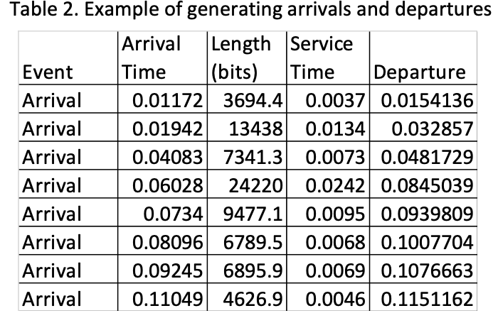
2. Packet departure: Calculate the departure time of a packet based on the state of the queue, i.e., whether the queue has packets or it is idle. If the queue has packets, then the departure time of a packet pk $t_{i}$ will be the departure time of the previous packet pk $t_{i - 1}$ plus the service time of pk $t_{i}$ . Note that the service time depends on the length of the packet, L, and the transmission rate, C, of the server. If the queue is idle, then the departure time of packet pk $t_{i}$ will be its arrival time plus its service time. See Table 2.
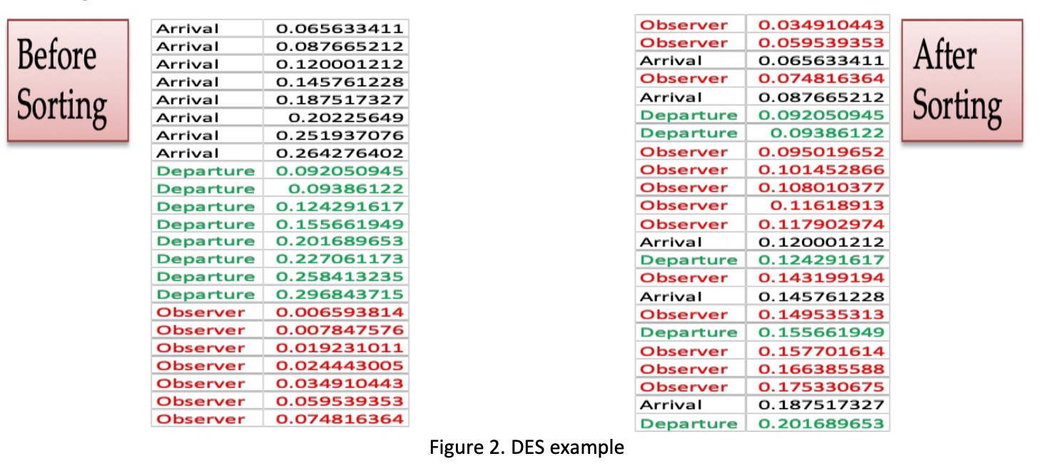
3. Observer: In order to monitor the queue, you need to generate observer events at which you are going to record the state of the queue. Generate a set of random observation times according to the packet arrival distribution with rate at least 5 times the rate of the packet arrival. At an observer event, you will record the state of the queue which can be done by recording the following: the time-average of the number of packets in the queue, $E [N]$ , the proportion of time the server is idle (i.e., the system is empty) $P_{I D L E}$ and in the case of a finite queue, the probability $P_{L OSS}$ that a packet will be dropped (due to the buffer being full when it arrives). The measurement and recording of the state should be performed such that we have statistically representative information on the performance that we are interested in. In order to record the state of the queue, you need to have three counters: $N_{a}$ = number of packet arrivals, $N_{d}$ = number of packet departures, and $N_{o}$ = number of observations. The onus is on you to find out how to use the previous three counters to calculate the state of the queue, i.e., $E [N]$ , $P_{I D L E}$ , and $P_{L OSS}$ (in case of finite queue). We typically assume that the observation is instantaneous (that is, there is no service time for observation).
After generating all the three events, put all the events in a list and sort them according to time as shown in the Fig. 2.

Start processing the events in order from DES. Based on the event type, you should update the three counters $N_{a}$ , $N_{d}$ and, $N_{o}$ . If the event is observer, calculate the performance metrics of interest, e.g., $P_{I D L E}$ , $P_{L OSS}$ . After an event has been processed, it should be deleted from DES.

4.6 Notations

$λ =$ Rate parameter
$L =$ Average length of a packet in bits
$α =$ Average number of observer events per second
$C =$ The transmission rate of the output link in bits per second
$ρ =$ Utilization of the queue (= input rate/service rate = $L λ / C$ )
$E [N] =$ Average number of packets in the buffer/queue
$P_{I D L E} =$ The proportion of time the server is idle, i.e., no packets in the queue is being transmitted
$P_{L OSS} =$ The packet loss probability (for M/M/1/K queue). It is the ratio of the total number of packets lost due to buffer full condition to the total number of generated packets

5 Report Requirements

Read all the questions in the report template document before you start designing your simulator.

Note that the questions build on each other. It is imperative that you ensure the code for each question is

working before moving on to the next, or you will compound your errors.

6 FINAL REPORT

Submit the following in a *.zip file to the dropbox on LEARN. Your zip file may not include subdirectories. It must be named

using your (maximum) 8-character UW ID plus the suffix _lab1.zip, such as “mstachow_lab1.zip”. Incorrectly named files will lose marks.

Source code with proper documentation/comments. Insufficient documentation will result in losing marks. This source code must be submitted as *.py files. Do not submit source code in your report!
Your filled in report template, submitted as a pdf. Submitting in any format other than pdf will result in lost marks.

You may be asked to give a demo of your simulator.

import random
import math
import matplotlib.pyplot as plt
 
class Event:
    def __init__(self, event_type, event_time):
        self.event_type = event_type
        self.event_time = event_time
 
# returns a single random sample drawn from an exponential random distribution
def exponential_random_var(lam):
    U = random.uniform(0, 1)
    return -math.log(1 - U) / lam
 
# generates samples from an exponential random distribution with lambda (q1)
def generate_samples(lam, num_samples):
    samples = [exponential_random_var(lam) for i in range(num_samples)]
 
    # mean and variance of the samples
    mean = sum(samples) / num_samples
    variance = sum((x - mean) ** 2 for x in samples) / num_samples
 
    # expected mean and variance
    expected_mean = 1 / lam
    expected_variance = 1 / (lam ** 2)
 
    print("Mean of samples: ", mean)
    print("Variance of samples: ", variance)
    print("Expected mean: ", expected_mean)
    print("Expected variance: ", expected_variance)
 
    # Plot histogram of the samples
    plt.hist(samples, bins=30, alpha=0.7, color='blue', edgecolor='black')
    plt.title('Histogram of Exponential Random Variables')
    plt.xlabel('Value')
    plt.ylabel('Frequency')
    plt.show()
 
def main():
    generate_samples(75, 1000)
 
if __name__ == "__main__":
    main()

Lab 2

Some commands to learn:

🪴 Avril Chen

Explorer