Dynamic Programming

First seen and learned in CS341 (Lecture 11)

Don’t be fooled by the name. Very misleading. Just a cool name.

Dynamic programming applies when the subproblems overlap, that is, when subproblems share sub-subproblems.

A dynamic-programming algorithm solves each sub-subproblem just once and then saves its answer in a table, thereby avoiding the work of recomputing the answer every time it solves each sub-subproblem.

Dynamic programming typically applies to optimization problems. Such problems can have many possible solutions. Each solution has a value, and you want to use a solution with the optimal (minimum or maximum) value. We call such a solution an optimal solution to the problem, as opposed to the optimal solution, since there may be several solutions that achieve the optimal value.

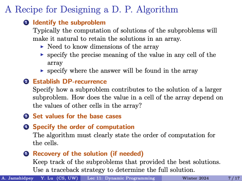
To develop such algorithm, follow four steps:

1. Characterize the structure of an optimal solution.
2. Recursively define the value of an optimal solution.
3. Compute the value of an optimal solution, typically in a bottom-up fashion.
4. Construct an optimal solution from computed information

Two uses for dynamic programming:

• Finding an optimal solution: We want to find a solution that is as large as possible or as small as possible.
• Counting the number of solutions: We want to calculate the total number of possible solutions.

From CS341

DP vs Greedy Algorithms

The Greedy algorithms we have seen usually require a way to order or pick the items. Once we find this way (which is sometimes more difficult then just ordering the items from largest to smallest and vice versa) and we can guarantee that picking items in this order / method will build our optimal solution / set, then we use the greedy strategy. 

A good example of a problem that we can use the greedy strategy is: Knapsack

• Given n items, each with a weight and a value, maximize the total value in your knapsack while staying under it’s capacity, W 
• Here, we are allowed to include fractions of the items.
• The solution: 
  • ordering: divide each item value by it’s weight (value per weight). Then pick items to go in the knapsack in the order of descending value per weight. Once an item will not fit, take the fraction of it that can fit and put it in and your done. 

We need Dynamic Programming when more “strategy” is involved: 

For example, O/1 Knapsack. It’s the same thing, but we can’t use fractions of items. As a result, if we were using our greedy strategy, we could get to the end and have extra space in the Knapsack. Sure, we may have chosen the items with the most value per weight, but maybe we have a lot of extra space that could have been utilized by smaller weight items with less value. So here, we need a different strategy.

So personally, I try to first apply a greedy strategy to solve the problem and then it usually becomes clear when the optimal solution depends on more than just the current item being added to the solution and also on past/future items.