CS341: Algorithms
A continuation of CS240 Everything can be found on Learn. Taught by Armin Jamshidpey in W2024. Really enjoyed this course.
Lecture notes from another prof: https://cs.uwaterloo.ca/~lapchi/cs341/notes.https://cs.uwaterloo.ca/~lapchi/cs341/notes.htmlhtml
Textbook CLRS is very good. Textbook answers: https://github.com/wojtask/clrs4e-solutions.
Midterm Midterm CS341
Final - Tuesday April 16 2024
Some information about the final exam:
- It covers Lec8-Lec18. The topics are mainly about greedy algorithms, dynamic programming, and NP-completeness. We won’t specifically ask a direct question about Lec1-Lec7 (which were tested for the midterm), but we assume knowledge from these lectures (e.g. we can use DFS to check whether a directed graph is acyclic, use BFS to compute shortest paths, etc) and you may need to use them.
The proof of the Cook-Levin Theorem will not be asked. From Lec17 and Lec18, you don’t need proofs.
-
No notes and books allowed. No electronic devices (e.g. calculators) allowed. There is no reference sheet.
-
You can assume the material in the notes without providing details. You can also assume the content in CS 240 and Math 239 without providing details. No other assumptions can be made without providing details, not from homework, tutorials, reference books, etc. For example, if we ask you a question that is from homework/tutorials, we expect you to answer this question from scratch (instead of saying that we have done it in homework/tutorials).
-
You will be given partial marks even though you do not know how to solve the problem completely (e.g. having a slower algorithm, having some rough ideas about the reductions, etc).
-
For preparation, go through the lecture notes, the homework, the tutorial notes, and the good problems in textbooks (CLRS, KT, DPV).
-
Make sure you read each question on the exam carefully and completely
Topics:
- Dijkstra’s algorithm
- Greedy algorithms
- MST
- Kruskal’s algorithm
- Dynamic Programming
- NP
Focus on later part of the course. Apparently L17 and L18 don’t need to know. Just know the NP-complete problems: https://piazza.com/class/lr45czd8jab7cz/post/1200
To review:
- Recursion tree
- Review midterm
- Do final practice problems
- Do all tutorials
- Focus on NP problem (they are going to ask at least one or two)
Concepts
Lecture 2
Lecture 3 - 4
- Master Theorem
- Recursion-Tree Method
- Recurrence Relations
- Karatsuba Algorithm
- Strassen Algorithm
- Median of medians
- Quickselect - selection algorithm
Lecture 5
Lecture 6
Lecture 7
Lecture 8
Lecture 9
Lecture 10
Lecture 11
- Dynamic Programming
- Interval Scheduling Problem
- Knapsack Problem
Lecture 12
Lecture 13
- Edit Distance
- Optimal Binary Search Trees
- Independent Sets in Trees
Lecture 15
Lecture 16
Lecture 17 and Lecture (don’t worry about it)
Lecture 3 - Divide an Conquer
Example - Counting inversions
Collaborative filtering:
- matches users preferences (movies, music, …)
- determine users with similar tastes
- recommends n ew things to users based on preferences of similar users
Goal: given an unsorted array , find the number of inversions in it.
Def
is an inversion if and
Example: with
A=[1,5,2,6,3,8,7,4], we get
Remark: we show the indices where inversions occur
Remark: easy algorithm (two nested loops) in
Lecture 4 - Divide and Conquer
- The Selection Algorithm We don’t choose the pivot randomly now.
How to find a pivot such that both
iandn-i-1are not too large?
 For each group, we spend to find the medians. Then we have to find the median of medians. Why?
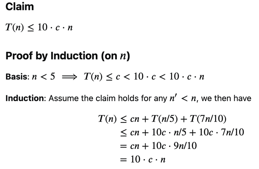
Why is the runtime of median of medians
O(n)?T(n) = T(n/5) + T(7n/10) + O(n) is the expression given in the slides T(n/5) and O(n) term is from finding median of medians in the groups of 5 This is from selectPivot() The current array is broken up into groups of 5 (takes O(1) time) There are n/2 groups of 5 Calling quickselect on an array of size 5 is fixed time operation (takes O(k) = O(1)) but there are n/5 groups so finding the median of every group of 5 will take O(n) time Thus the terms T(n/5) + O(n)
T(7n/10) is the worst case for the size of the next array This worst case is bounded by the pivot selection from selectPivot(), proof of this in slides (the maximal size of the next recursive call’s array is 7n/10)
Its an induction proof to show why
Note, in quicksort, you have to sort both sides of the array after the pivot step. In median of medians, after the pivot step, you only have to consider one part of the array, the one that has the median.
and are the sizes of the right and left subarrays. and .
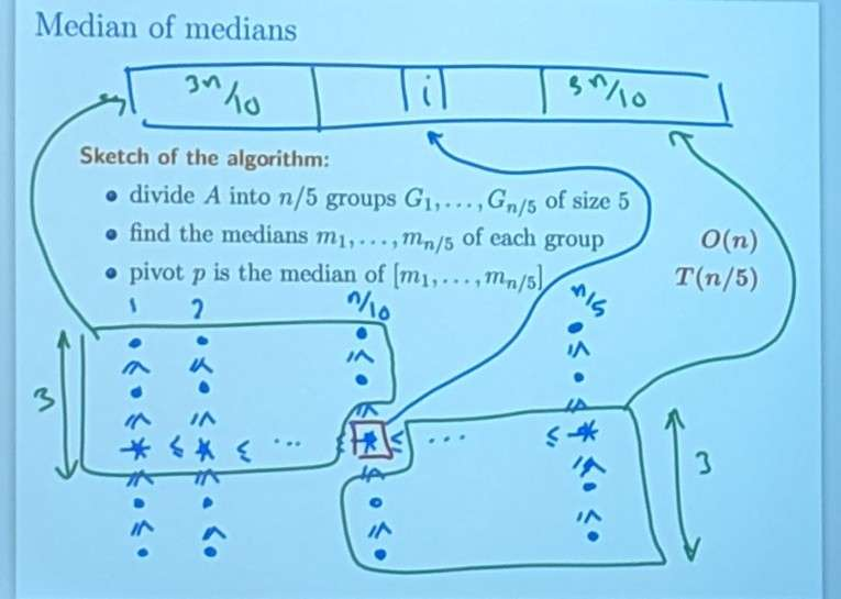 He’s not sorting each group. After finding the median of medians, you can reorder the element (the columns) in the picture.
After calling the partition algorithm, we get an array where the median of medians is at some index . The values in the green area is smaller than the median of medians. All these values goes before the index. Same argument can be done to the bottom right corner. In the green box, the elements are going to be larger and will appear on the left in the array .
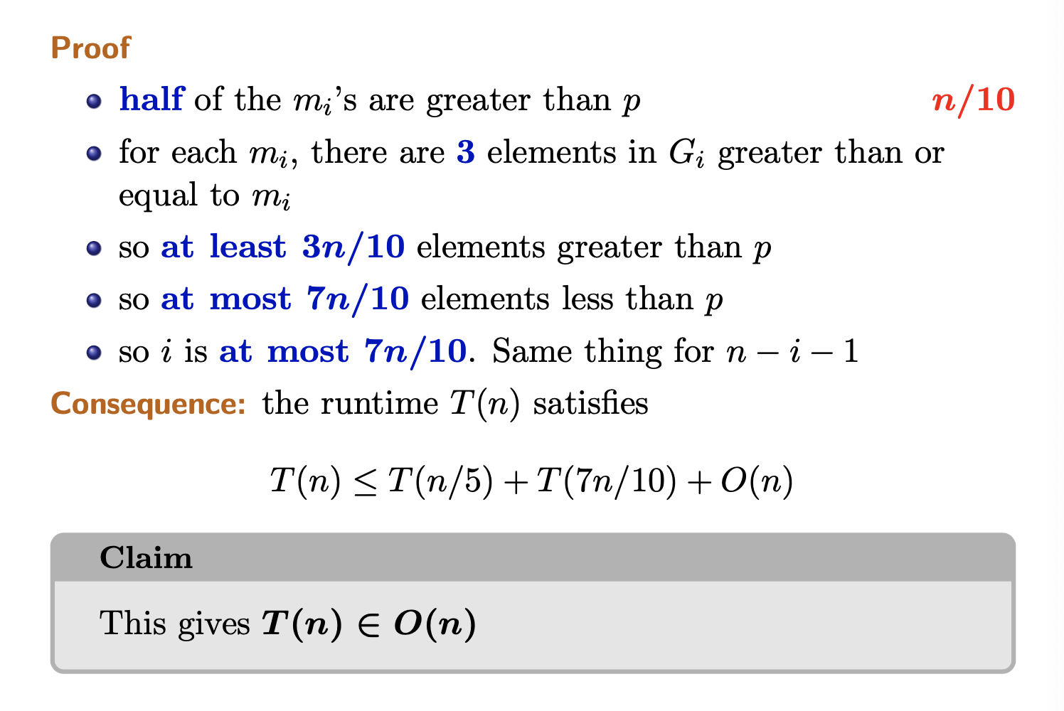
- is the runtime to find the median of medians. we ensure that the pivot chosen is at least in the middle 30%
- Because in the median of medians algorithm, the key idea is to ensure that the pivot chosen is not too small or too large compared to the rest of the elements in the array. Specifically, the pivot selected by the median of medians algorithm is guaranteed to be within the middle 30% of the sorted order of the array.
- Worst case is the recursive call , because it’s quick select and not quick sort. only 7 branches and we ignore the other 3 branches? since quickselect does not partition the array into equal parts, rather it focuses on only one side of the pivot (where the desired element should be located). so worst case, only one side of the array is considered
- is the extra operations to be done, in this case, partitioning We can prove the runtime to be
Why are we grouping them in groups of 5?
Might not work with other grouping numbers. We will see later.
Module 3
Lecture 5 - Breadth First Search
not gonna do bfs and undirected graphs
Goals:
-
basics on undirected graphs
-
undirected BFS and applications (shortest paths, bipartite graphs, connected components)
-
undirected DFS and applications (cut vertices)
-
basics on directed graphs
-
directed DFS and applications (testing for cycles, topological sort, strongly connected components)
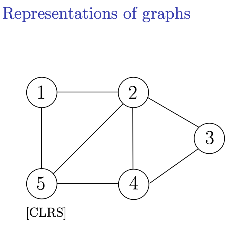
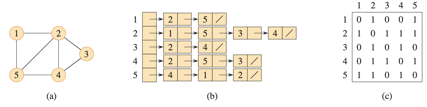
Draw the representation of an undirected graph as an adjacency list and matrix for this graph
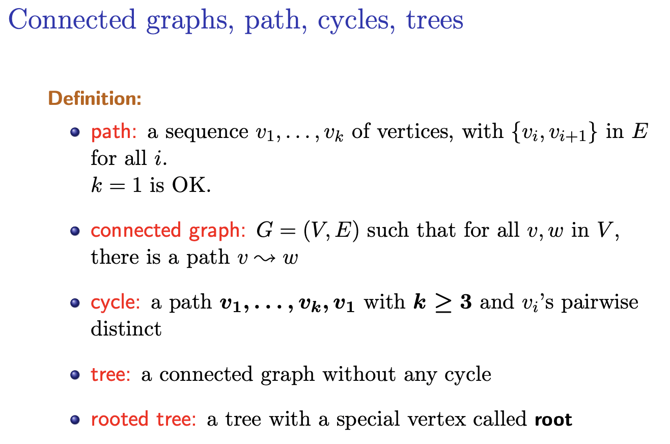
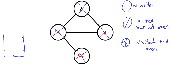
Some definitions
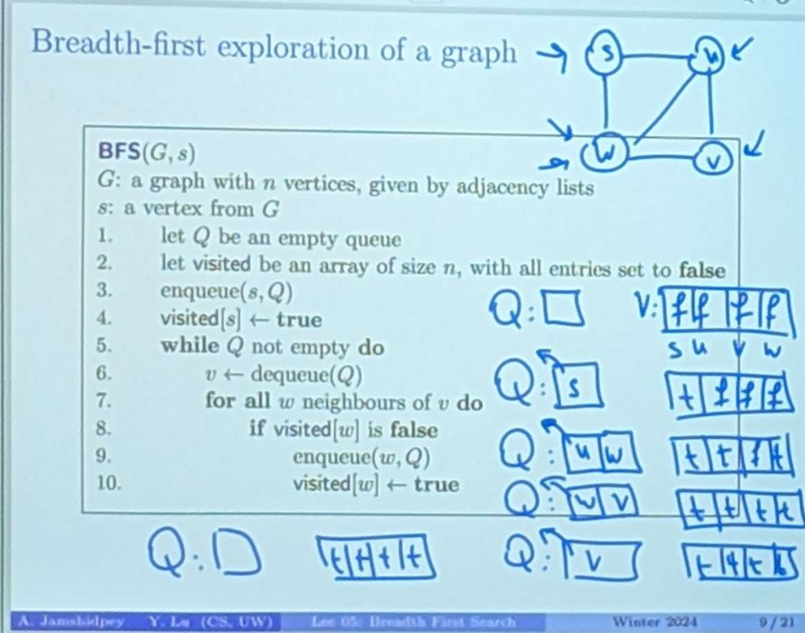
BFS
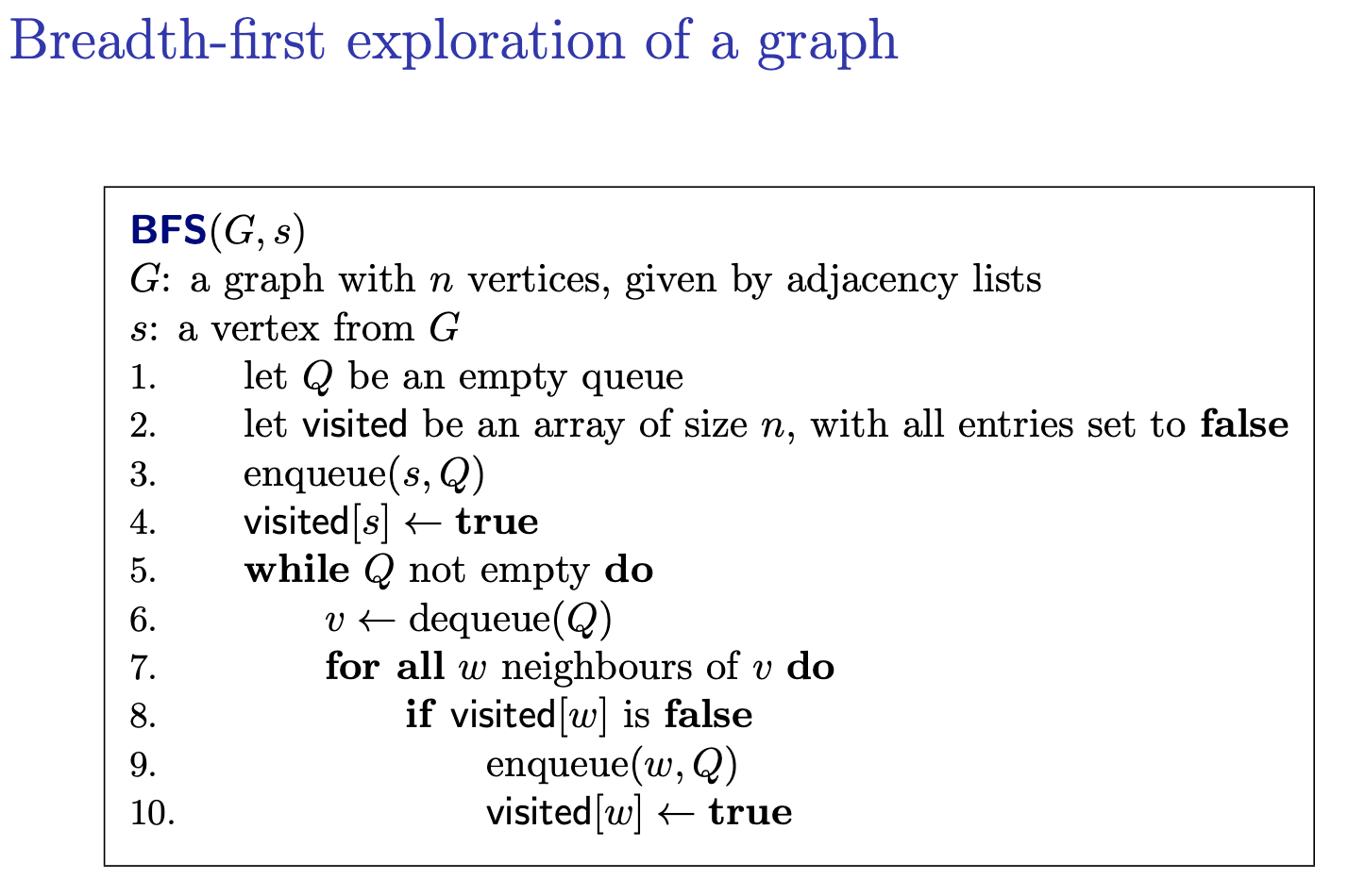
As long as the queue is not empty based on the order of queue. Take things out. and look at all the neighbours. If the neighbours is not visited, we enqueue it.
Time Complexity
Analysis:
- each vertex is enqueued at most once
- so each vertex is dequeued at least once
- so each adjacency list is read at most once (since we visit all the neighbours of a vertex only if it has not been visited)
For all , write number of neighbours of length of degree of .
cf. the adjacency array has cells (Handshaking Lemma)
Total:
Breadth-first exploration idea: start from yourself, and expand.
Thu Jan 25, 2024
To dequeue you need to visit all of the neighbours.
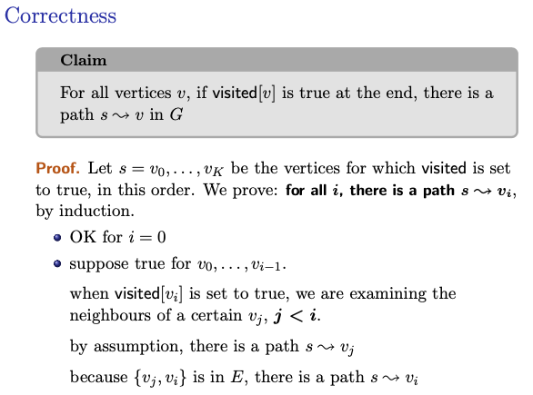
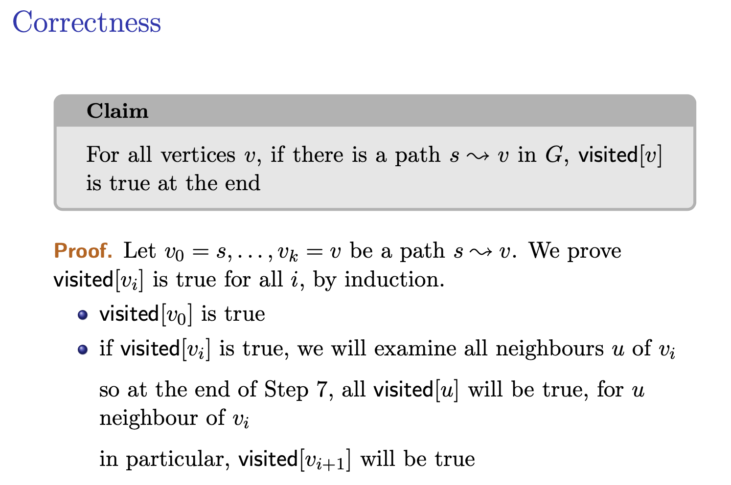
Use induction, assume the statement holds for vi, we want to show that vi+1 is visited. If vi is visited, it means that it enqueue. But to enqueue, we need to dequeue and to dequeue we visit all of the neighbours. And since vi+1 is a neighbour of vi, therefore vi+1 is visited.
Lemma
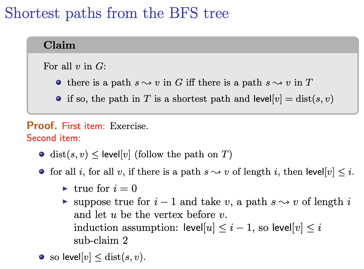
For all vertices , there is a path v in if and only if is true at the end.
Applications
- testing if there is a path v
- testing if is connected in .
To check if a graph is connected, we need to run DFS.
To test if the and : is the dominant term.
Exercise
For a connected graph, .
Thu Jan 25, 2024
I visit some node , but why do we do that in BFS?
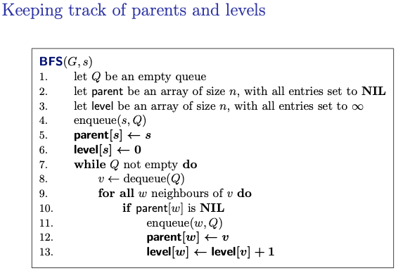
If I have a parent array, do we still need a visited array?
- No, we can just go check the parent array and check if it’s null or it visited the child.
In the textbook, they use predecessor to mean parent. It’s more general.
Based on this algorithm, we can form a tree!
is the parent.
Example for the algorithm (i’ve recorded the whole process):
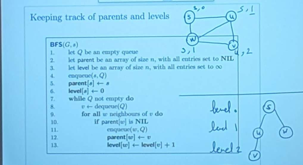
BFS Tree
BFS Tree
Definition: the BFS Tree is the subgraph made of
- all such that
- all edges , for as above (except )
Claim
The BFS tree is a tree.
Proof: by induction on the vertices for which is not NIL.
- when we set , only one vertex, no edge.
- suppose true before we set was in before, was not, so we add one vertex and one edge to , so remains a tree.
Remark: we make it a rooted tree by choosing as a root.
Shortest paths from the BFS tree
Sub-claim 1
The levels in the queue are non-decreasing
Proof: Exercise
Sub-claim 2
For all vertices if there is an edge {}, then .
Proof.
- if we dequeue before , (sub-claim 1)
- if we dequeue before , the parent of is either , or was dequeued before in any case, (sub-claim 1) but , so OK
gap-in-knowledge don’t really understand the proof of sub-claim 2. Does it mean either is the parent of or someone else is the parent of and got dequeue earlier, before dequeueing . Therefore, level of u + 1 is definitely bigger or equal to level of v, since it’s above . Doesn’t make sense, i got it wrong? if we dequeue u before, doesn’t it mean that u is lower level than v? Omg notice that there is an edge {u,v}. But still why is it level of u + 1 is greater or equal to level of v? Is level 1 higher than level 2? I think I’m misunderstanding the lower and higher. If 1 is higher level then I got it right…
 What is ? The BFS Tree I assume.
I’m very confused: I have recordings.gap-in-knowledge
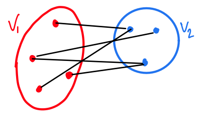
Bipartite Graph
A graph , is bipartite if there is a partition such that all edges have one end in and one end in .
Using BFS to test bipartite-ness
Claim
Suppose connected, run BFS from any , and set
- vertices with odd level
- vertices with even level
Then is bipartite if and only if all edges have one end in and one end in (testable in )
Proof. obvious For , let be a bipartition. Because paths alternate between :
- ( vertices with odd level) is included in (say)
- ( vertices with even level) is included in So and
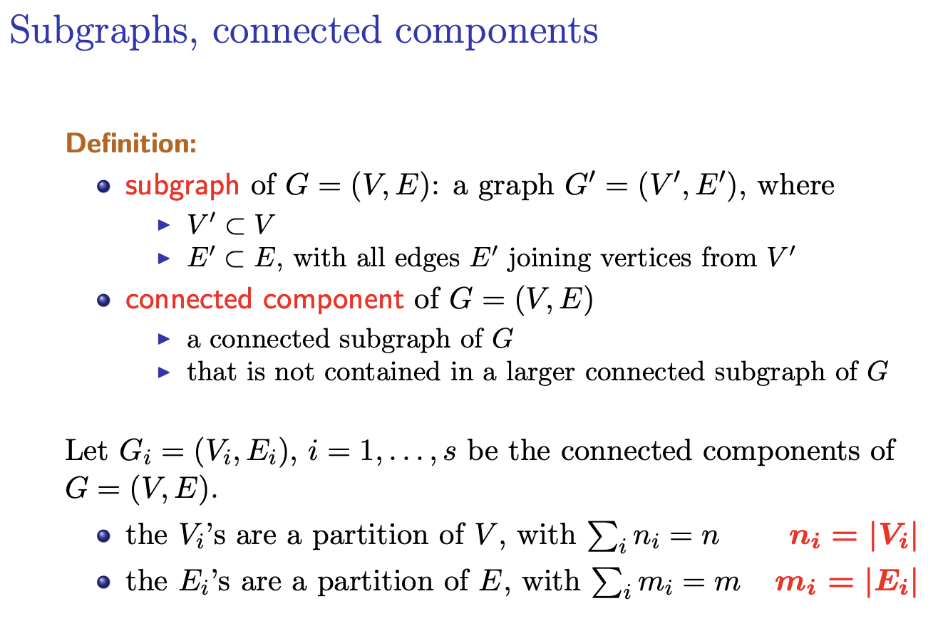
Computing the connected componentsto-understand
Idea: add an outer loop that runs BFS on successive vertices
Exercise
Fill in the details.
Complexity:
- each pass of BFS , if is the th connected component
- total
Slide explained
It’s just giving the idea of how to find the connected components of an undirected graph. You run a BFS, and then you’re done you’ve visited all the vertices in that component. So you just need to find an unvisited vertex (which means it will be in another component) and then run BFS on that vertex again. You keep doing this until you visit every vertex.
Chatgpt: The approach described is a common method for computing the connected components of an undirected graph using BFS (Breadth-First Search). Let’s break down the steps:
- Initialize: Start with an empty list to store the connected components.
- Outer Loop: Begin an outer loop that iterates over all vertices of the graph. For each vertex, if it has not been visited yet, it means it belongs to a new connected component.
- BFS: Perform a BFS traversal starting from the current unvisited vertex. This BFS traversal will visit all vertices reachable from the current vertex, which form one connected component of the graph.
- Store Component: After completing the BFS traversal, all vertices visited during this traversal belong to the same connected component. Add these vertices to the list representing the current connected component.
- Repeat: Continue the outer loop to find the next unvisited vertex in the graph. This vertex will belong to a new connected component. Repeat steps 3-4 for this vertex.
- Termination: Once all vertices have been visited and assigned to connected components, the process ends.
Let’s analyze the complexity:
- BFS Complexity: Each pass of BFS on a connected component takes time, where is the number of vertices and mimi is the number of edges in the th connected component.
- Total Complexity: Since we perform BFS on each connected component separately, the total complexity is the sum of the complexities of all BFS traversals, which is , where is the total number of vertices and is the total number of edges in the graph.
This approach efficiently computes the connected components of an undirected graph by systematically exploring each component using BFS. It’s a fundamental technique in graph theory and is often used in various applications such as network analysis, social network analysis, and image processing.
Lecture 6 - Depth-First Search
Going depth-first
The idea:
- travel as deep as possible, as long as you can
- when you can’t go further, backtrack
DFS implementations are based on stacks, either implicitly (recursion) or explicitly (as with queues for BFS).
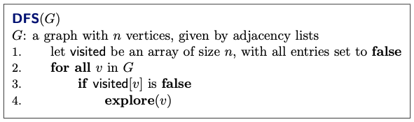
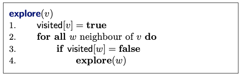
Recursive Algorithm:
Remark: can add parent array as in BFS. What does that mean?:
- Adding a parent array in DFS, similar to BFS, means keeping track of the parent of each vertex encountered during the traversal. In BFS, the parent array is used to reconstruct the shortest paths from the source vertex to all other vertices in the graph. However, in DFS, the parent array serves a slightly different purpose.
- In DFS, the parent array can be used to represent the DFS tree or forest. Each time a vertex is visited and explored, the parent of its neighbouring vertices becomes , since is the vertex from which was discovered. Therefore, by maintaining this information in the parent array, we can construct the DFS tree rooted at any vertex. Here’s how it works:
- Initialize a parent array of size , where nn is the number of vertices in the graph. Initially, all entries in the parent array are set to a special value (e.g., ) to indicate that the vertices have no parent.
- During the DFS traversal, when exploring a vertex , mark as visited (i.e., ) and iterate through all its neighbours .
- For each neighbour , if has not been visited yet, set its parent in the parent array to (i.e., ). By the end of the DFS traversal, the parent array will represent the DFS tree or forest, where each vertex (except the root(s)) has a parent that discovered it during the traversal. This information can be useful for various purposes, such as finding paths in the DFS tree, detecting cycles, or performing other graph-related algorithms.
Notice, it is recursively calling on explore().
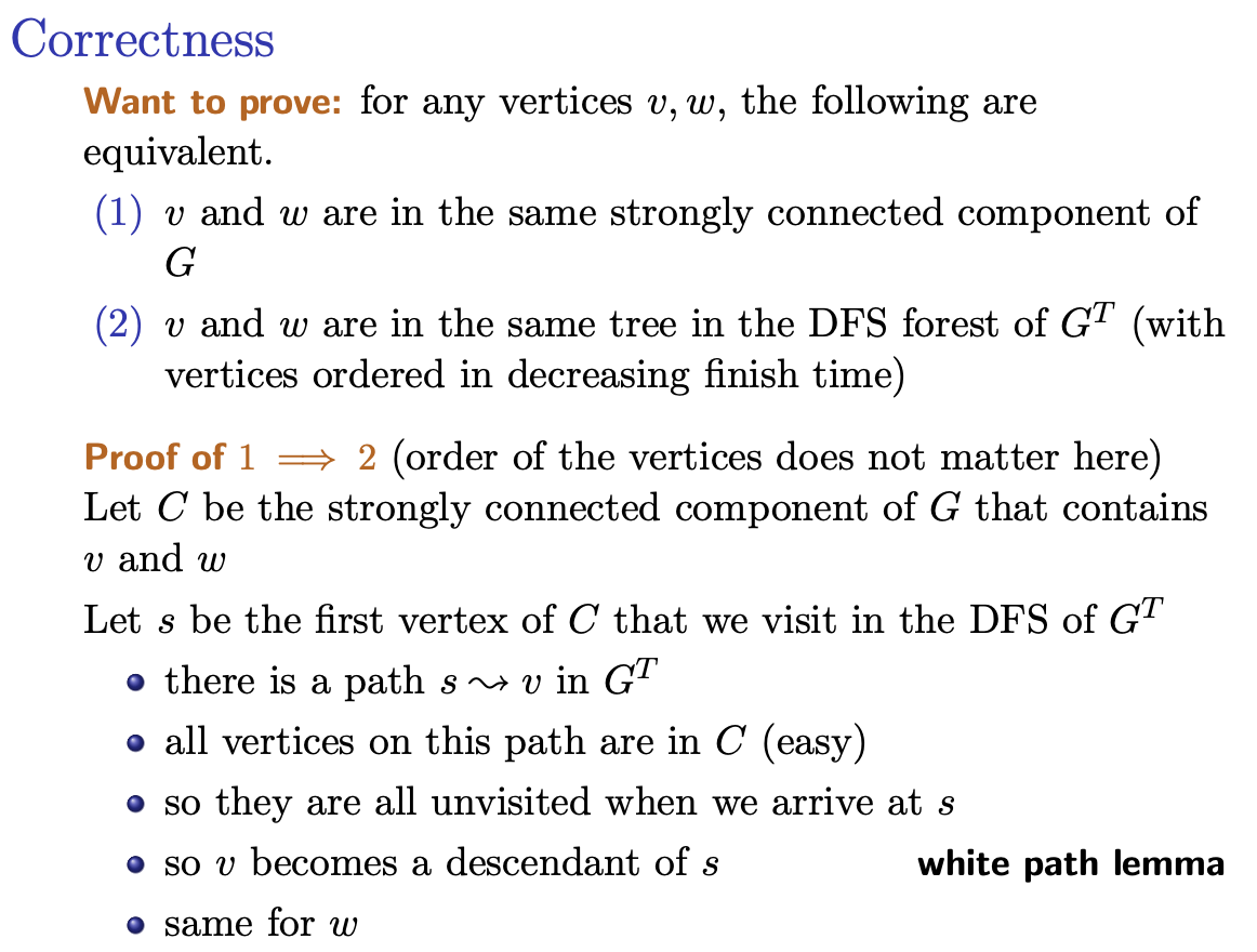
Claim ("white path lemma")
When we start exploring a vertex , any that can be connected to by an unvisited path will be visited during explore().
Proof: Let’s prove this lemma by contradiction. Suppose there exists a vertex that can be reached from by an unvisited path but is not visited during the exploration of .
- Initialization: We begin the DFS traversal with all vertices marked as unvisited.
- Exploration of : When the DFS algorithm starts exploring vertex , it marks as visited. Then, for each neighbour of , if has not been visited yet, DFS explores .
- Contradiction: However, by the nature of DFS, when exploring , all its neighbours are visited recursively. Therefore, if is reachable from , it must be a neighbour of or a neighbour of a neighbour of , and so on. Since DFS explores all neighbours of and their neighbours, should have been visited during the exploration of . But our assumption states otherwise, leading to a contradiction.
Hence, the assumption that there exists a vertex reachable from via an unvisited path but not visited during the exploration of is false. Therefore, any vertex that can be connected to by an unvisited path will indeed be visited during the exploration of . This completes the proof of the “white path lemma”.
Basic property:
Claim
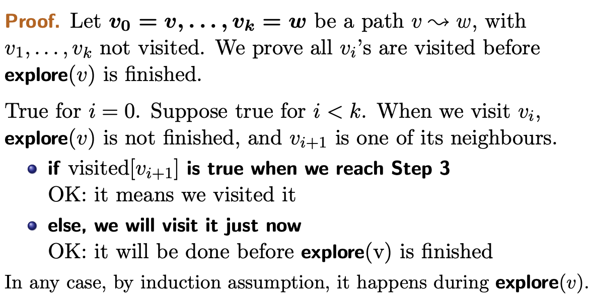
If is visited during explore(), there is a path .
Proof: Same as BFS.
The proof is straightforward and relies on the nature of DFS exploration. During the DFS traversal, when exploring vertex , DFS recursively visits all vertices reachable from in the graph.
- Initialization: The DFS traversal begins with the starting vertex marked as visited.
- Recursive Exploration: For each neighbour of , if has not been visited yet, DFS explores . This process continues recursively until all reachable vertices from have been visited.
- Vertex : If vertex is visited during the exploration of , it means that is reachable from in the graph.
- Path from to : Since is visited during the exploration of , there must be a path from to in the graph. This path is formed by the sequence of edges traversed during the DFS traversal.
Therefore, if vertex is visited during the exploration of vertex in DFS, then there exists a path from to in the graph. This completes the proof of the claim.
Consequences:
- Previous properties: after we call explore at in DFS, we have visited exactly the connected components containing .
- Since it recursively explores all the vertices in the connected component
- Shortest paths: no
- unlike bfs, it does not get you the shortest path
- Runtime: still
Trees, forest, ancestors and descendants Previous observation:
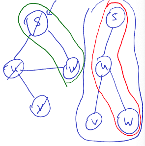
- DFS() gives a partition of into vertex-disjoint rooted trees (DFS forest)
- What does this mean>
Definition. Suppose the DFS forest is and let be two vertices
- is an ancestor of if they are on the same subtree in the DFS forest and is on the path root
- equivalent: is a descendant of if
- belongs to the subtree rooted at in the DFS forest
- equivalent as saying is the ancestor of
In other words, in a DFS forest:
- An ancestor of a vertex is any vertex that lies on the path from the root of the subtree containing the vertex to the vertex itself.
- A descendant of a vertex is any vertex within the subtree rooted at the vertex.
Key Property
Claim
All edges in connect a vertex to one of its descendants or ancestors.
So, there is no edge from subtree to subtree within :
Proof. Let {} be an edge, and suppose we visit first. Then when we visit , is an unvisited path between and , so will become a descendant of (white path lemma).
White Path Lemma: According to the white path lemma, any vertex that can be connected to by an unvisited path will be visited during the exploration of .
Back edges
A back edge is an edge in connecting an ancestor to a descendant, which is not a tree edge.
Observation: All edges are either tree edge or back edges (key property).
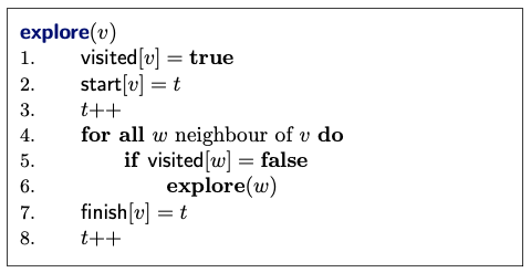
Start and finish times
Set a variable to 1 initially, create two arrays start and finish, and change explore:
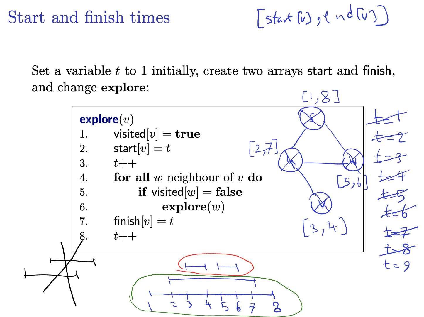
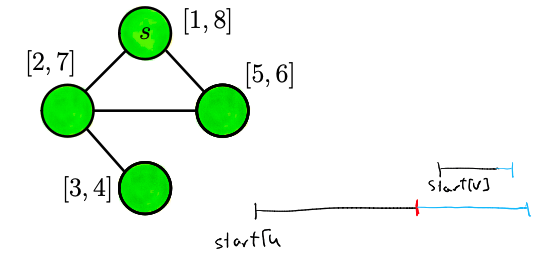
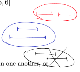
Example:
Observation:
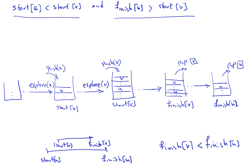
- these intervals are either contained in one another, or disjoint
- if , then either or .
- Basically saying that they can’t cross each other, either u finishes before v starts, or u finishes then v finishes.
Proof: if , we push on the stack while is still there, so we pop before we pop .
Cut vertices
Cut vertices
For connected, a vertex in is a cut vertex if removing (and all edges that contain it) makes disconnected. Also called articulation points
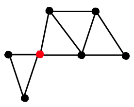
Finding the cut vertices ( connected)
Setup: we start from a rooted DFS tree , knowing parent and level.
Warm-up
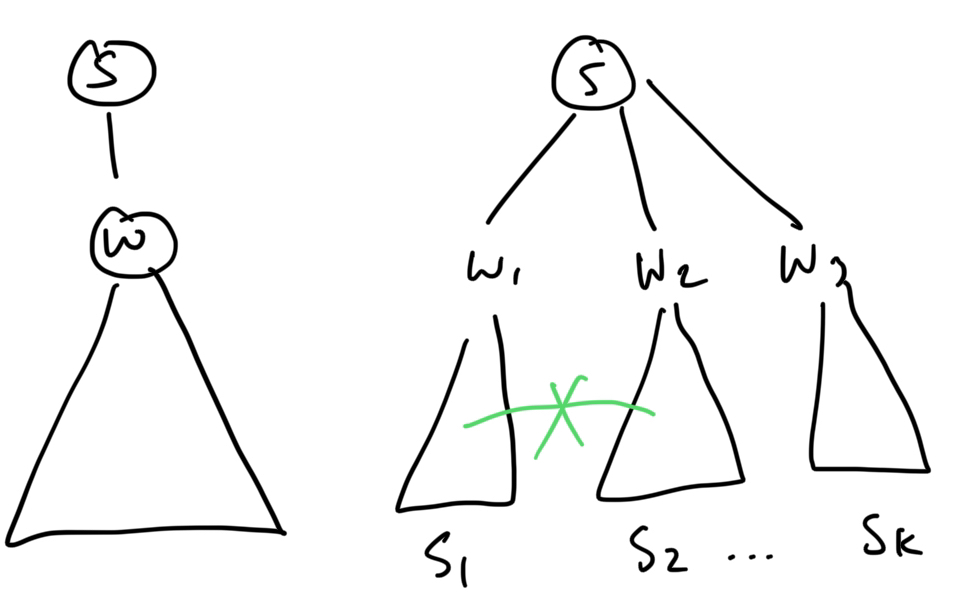
The root is a cut vertex if and only if it has more than one child.
Proof.
-
if has one child, removing leaves connected. So is not a cut vertex.
-
suppose has subtrees .
Key property: no edge connecting to for . So removing creates connected components.
Now, we want to investigate the problem of finding cut vertices which ARE NOT the root.
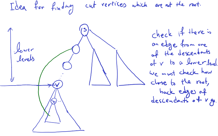
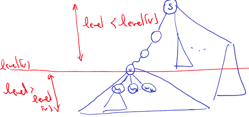
Finding the cut vertices (
Gconnected)Definition: for a vertex , let
{ {} edge}
{ descendant of }
- a(v) is the lowest level (highest in the tree) of all nodes directly connected to v.
- m(v) is the minimum a(w) value for all w; w is a descendant of v.
- ooo it considers all the descendants of , so basically any descendants of
- I interpret a(v) as the “highest link” that v has, while m(v) is the highest link that v’s subtree has.
In simple words:
- is the smallest level of all of ‘s neighbours
- is the smallest level of any neighbour of a descent of .
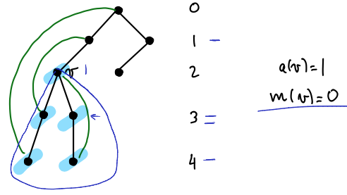
- Try calculating and and see if your results match the answers shown to the right of the diagram above!
Using the values
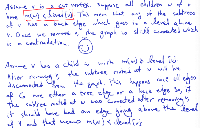
Claim
For any (except the root), is a cut vertex if and only if it has a child with .
Proof.
- Take a chid of , let be the subtree at .
- If , then there is an edge from to a vertex above . After removing , remains connected to the root.
- If , then all edges originating from end in . Proof: any edge originating from a vertex in ends at a level at least , and connects to one of its ancestors or descendants (key property).
Computing the values Observation:
- if has children , then {}
Conclusion:
- computing is
- knowing all , we get in
- so all values can be computed in (remember when connected)
- testing the cut-vertex condition at is
- testing all is
and are used for the children on a vertex which we are about to check if it is a cut vertex or not. The value gives the lowest level of all neighbours of , this counts for checking to see if a tree rooted at a child of a vertex will become disconnected or not.
Exercise: write the pseudo-code
1. Perform a DFS traversal on the graph G starting from any vertex (e.g., the root vertex).
2. During the DFS traversal, maintain the following information for each vertex v:
   - level[v]: the level of vertex v in the DFS tree
   - a[v]: the minimum level reachable from vertex v along edges in the DFS tree
   - m[v]: the minimum of a[v] and the values m[w] for all children w of v
3. Update a[v] and m[v] as follows:
   - When exploring a vertex v:
     - Set level[v] = t (where t is the current time)
     - Increment t
     - Set a[v] = level[v]
     - For each child w of v:
       - Recursively explore w
       - Update m[v] = min(a[v], m[v], m[w])
4. After the DFS traversal completes, iterate through all vertices v:
   - If v is not the root vertex and m[v] >= level[v], v is a cut vertex
5. The overall time complexity of this approach is O(m), where m is the number of edges in the graph.
Some questions:
- Running BFS also works exactly the same for finding cut vertices as running DFS right?
- Consider the 4-cycle, in the BFS tree, the claim would tell you that there is a cut vertex, but there is no cut vertex.
- I think this is because you can have edges to other subtrees in a BFS tree but this is impossible in a DFS tree.
Lecture 7 - Directed Graphs
Tue Feb 6 2024
Directed Graph
as in the undirected case, with the difference that edges are (directed) pairs
- edges are also called arcs
- usually, we allow loops, with
- is the source node, is the target
- a path is a sequence of vertices, with in for all . is OK.
- a cycle is a path
- a directed acyclic graph (DAG) is a directed graph with no cycle
Definition:
- the in-degree of is the number of edges of the from
- the out-degree of is the number of edges of the form
Data structures:
- adjacency lists
- adjacency matrix (not symmetric anymore)
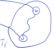
BFS and DFS for directed graphs The algorithms work without any change. We will focus on DFS.
Still true:
- we obtain a partition of into vertex-disjoint trees
- when we start exploring a vertex , any with an unvisited path becomes a descendant of (white path lemma)
- properties of start and finish times
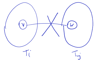
But there can exist edges connecting the trees
T_i.
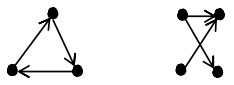
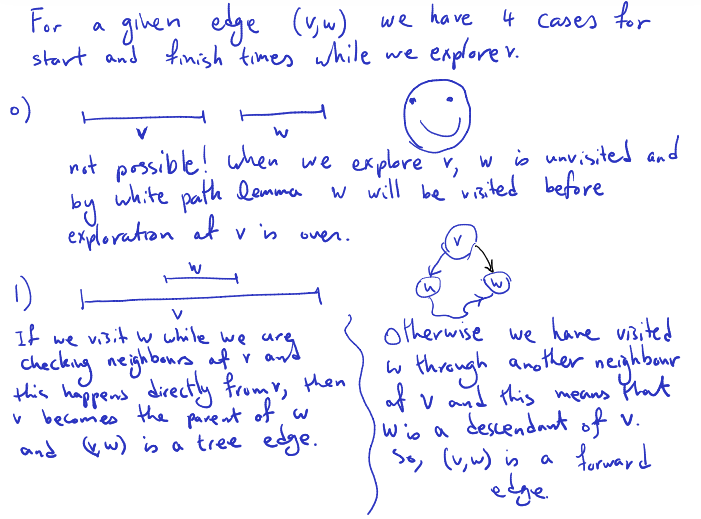
Classification of edges Suppose we have a DFS forest. Edges of are one of the following:
- tree edges
- A tree edge in the context of a DFS (Depth-First Search) forest of a directed graph is an edge that is part of the DFS tree itself. In other words, during the DFS traversal of the graph, when exploring a vertex , if a directed edge leads to a vertex that has not been visited yet, this edge becomes a tree edge and contributes to the construction of the DFS tree.
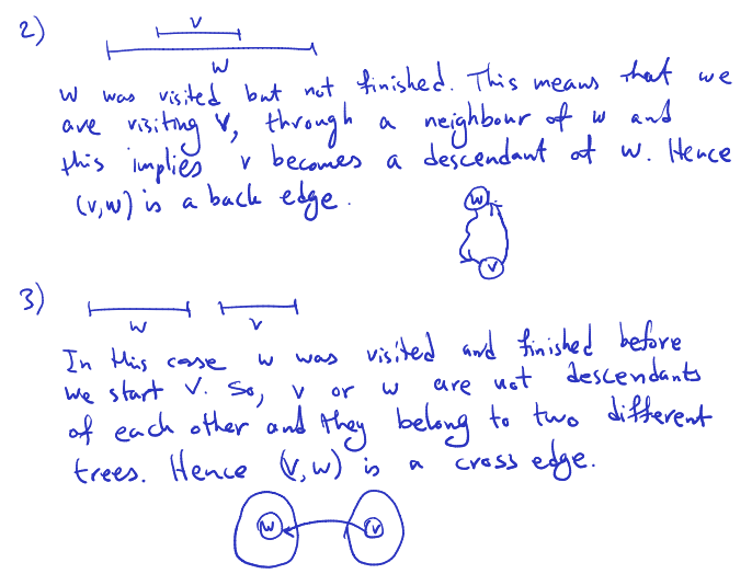
- back edges: from descendant to ancestor
- forward edges: from ancestor to descendant (but not tree edge)
- cross edges: all others
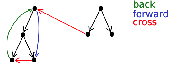
In this picture, if we were to start at node 1 (the node on the right) then the cross edge would become a tree edge correct?
So the classification of edges is not absolute but depends on where you start the DFS? yes
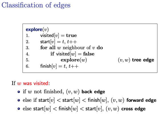
explore(v)
	visited[v] = true
	start[v] = t, t++
	for all w neighbour of v do
		if visited[w] = false
			explore(w)                      (v,w) tree edge
	finish[v] = t, t++
If was visited:
- if not finished, back edge
- Case 1: is visited and not finished yet:
- If vertex has already been visited but not yet finished (i.e., the DFS traversal is still exploring its descendants), and is an ancestor of , then the edge is considered a back edge.
- This condition indicates that is a descendant of in the DFS tree, and completes a cycle by connecting back to one of its ancestors .
- Case 1: is visited and not finished yet:
- else if forward edge
- else cross edge
- Case 1: : In this scenario, vertex was visited and finished before vertex was started. However, is not an ancestor of because . Therefore, the edge forms a cross edge.
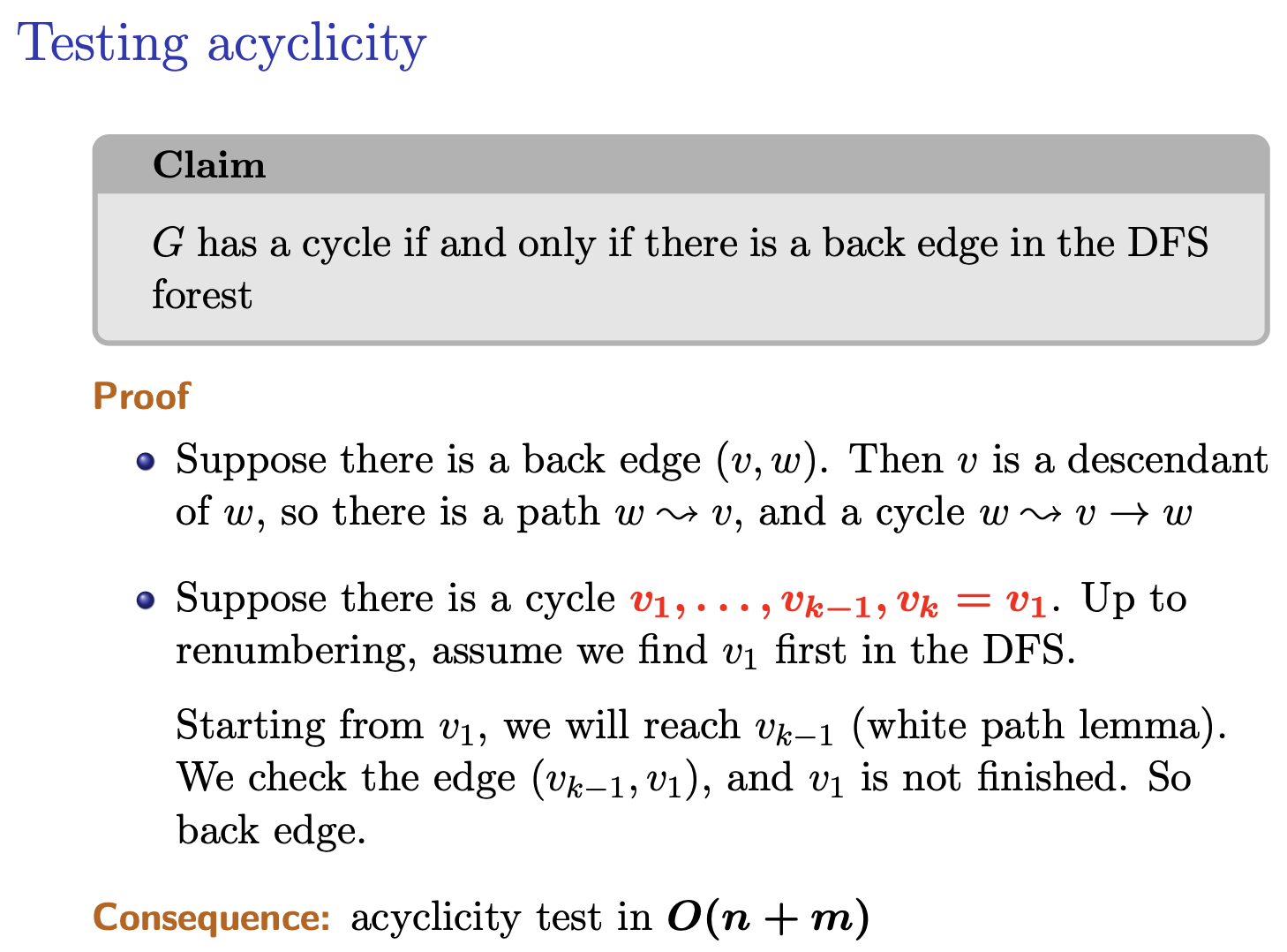
Testing Acyclicity
Claim
has a cycle if and only if there is a back edge in the DFS forest
Proof: : Since there is a back cycle, we have an edge from a descendent to an ancestor. So we have a cycle . Assume has a cycle , . Without loss of generality, we can assume we visit first (in the cycle).
At the time we start , the path is unvisited. By the white path lemma, we will visit before we finish . Hence becomes a descendent of and () is a back edge.
Topological Ordering
Topological ordering
Definition: Suppose is a DAG. A topological order is an ordering < of such that for any edge , we have .
No such order if there are cycles.
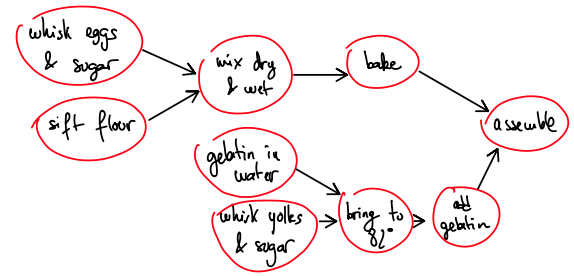
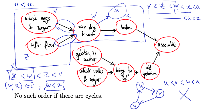
Need to write a topological ordering in a line. If two nodes are not connected, we have a choice to which one to write first.
There is no uniqueness. It gives you one of the topological ordering. Prof gave the analogy of prerequisites of the courses. You are in trouble if you have a cycle. No topological ordering???
In-degree node 0, good idea to put it first in your topological ordering. Same thing with out-degree node of 0 to be the last one.
Proposition:
Gis a DAG if and only if there is a topological ordering onv.
is a DAG There is topological ordering on . (It is an if and only if theorem, but prof just showed one way) (Not a proof (sketch)): Claim: must have at last one vertex with in degree 0.
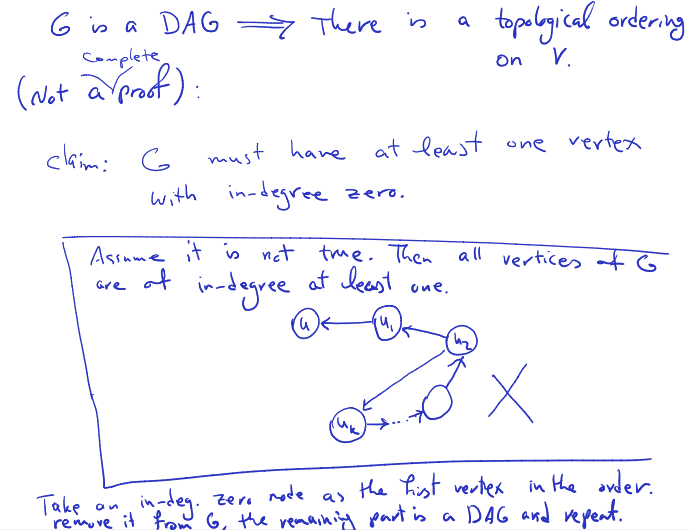
Assume it is not true. Then all vertices at are at in-degree at least one. Take an in-degree 0 node as the first vertex in the order remove it from , the remaining part in a DAG and repeat. At some point, we need to use one of the nodes used to have an edge going in the node at the start.
So we’ve found a contradiction. If we have a DAG, there must have a topological ordering.
From a DFS forest
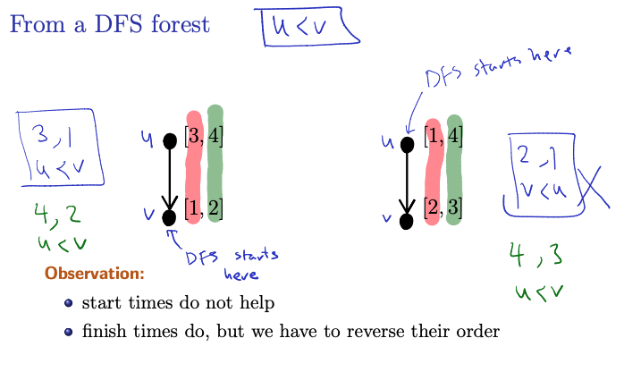
Observation:
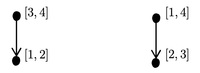
- start times do not help
- finish times do, but we have to reverse their order!
Left: is our topological order. we have 3,1 and Right: 2,1 Start time is not something we can rely on.
What about finish time? Left: 4,2 and Right: 4, 3 and
Claim
Suppose that is ordered using the reverse of the finishing order: .
This is a topological order.
SO: Definition of Topological Order: In a topological order, for every directed edge , vertex comes before vertex .
- Using Finish Times:
- In a DFS traversal, finish times indicate when vertices are finished being explored and all their descendants have been visited.
- We consider the reverse of the finishing order, so that vertices with later finish times come before vertices with earlier finish times. This makes sense, since if there is a topological order, there is gonna be a start, and we explore all the descendants starting from that node. It will finish last. Recursively go up.
Proof: Look at notes

- In a directed acyclic graph (DAG), there cannot exist a path from vertex to vertex if is discovered before during a DFS traversal. This is because if there were such a path, it would create a cycle in the graph, contradicting the acyclic property of the graph.
Topological order in .
Strong Connectivity
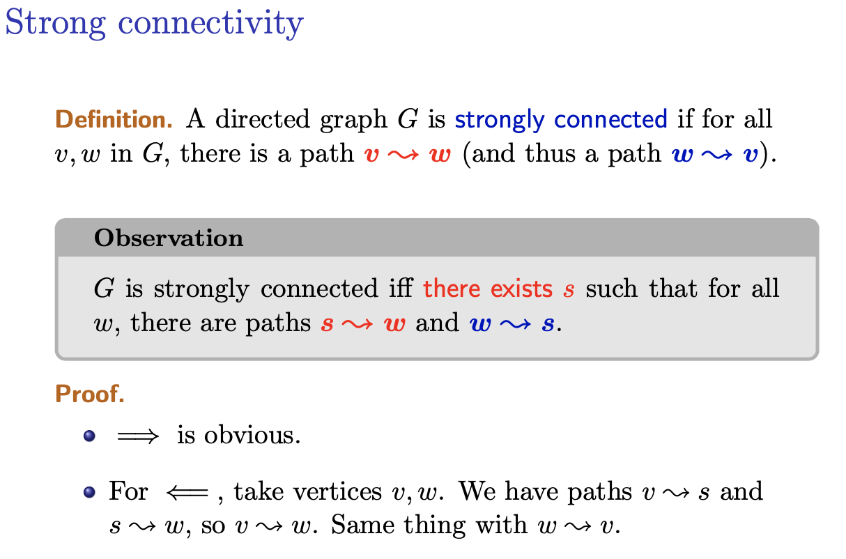
A directed graph is strongly connected if for all in , there is a path (and thus a path ).
Observation
is strongly connected there exists such that for all , there are paths and .
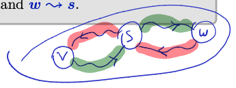
Proof:
- is obvious
- For , that vertices . We have paths and , so . Same thing with .
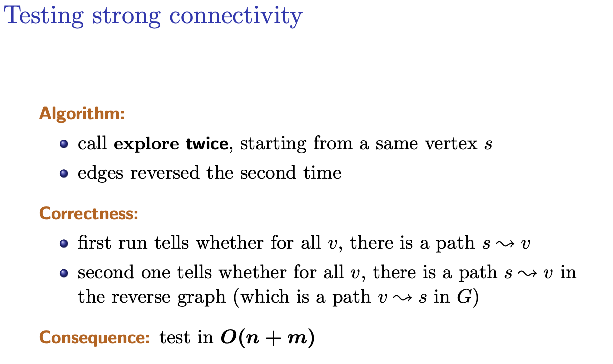
Algorithm:
- Perform a DFS exploration starting from vertex on the original graph .
- Perform another DFS exploration starting from vertex , but this time on the reverse graph , where all edges are reversed.
- If both DFS explorations reach every vertex in the respective graphs, then the graph is strongly connected.
Correctness:
- The first DFS exploration ensures that there is a path from to every other vertex in the original graph .
- The second DFS exploration, conducted on the reverse graph , ensures that there is a path from every vertex back to in the original graph , because reversing the edges effectively explores paths from every vertex back to in .
- Therefore, if both DFS explorations are successful, it implies that there exists a path from to every vertex and from every vertex back to , establishing strong connectivity.
Consequences:
- The algorithm tests for strong connectivity in time complexity, where is the number of vertices and is the number of edges in the graph.
- This approach provides an efficient way to determine whether a directed graph is strongly connected, which is essential for various applications and algorithms that rely on strong connectivity information.
If you give a direct graph and we take the reverse, we get a reverse graph where each edge is reversed. First run without reversing. Second run reverse and run DFS on the same node but on the reverse graph.
In G(T) is reversed, if we run DFS on this graph, there is a path
Have we considered the runtime of reversing the graph?
Might be asked on the midterm?? Do it in linear time. Prof only showed that it is in , but didn’t show the runtime to take to reverse a graph. Look
Approach to Reverse a Graph Efficiently:
- Original Graph Representation:
- Let’s assume the graph is represented using an adjacency list for each vertex, where each list contains the vertices adjacent to the corresponding vertex.
- Reverse Graph Representation:
- To reverse the graph, we need to reverse the direction of each edge. This essentially means swapping the source and target vertices for each edge.
- We can achieve this by creating a new reversed graph and populating its adjacency lists accordingly.
- Efficient Reversal:
- We can reverse the graph in linear time by iterating through each vertex and its adjacency list in the original graph.
- For each edge (u,v)(u,v) in the original graph, we add an edge (v,u)(v,u) to the corresponding adjacency list in the reversed graph.
- This process takes O(n+m)O(n+m) time, where nn is the number of vertices and mm is the number of edges in the original graph Runtime Analysis:
- The time complexity of reversing the graph is O(n+m)O(n+m), where nn is the number of vertices and mm is the number of edges in the original graph.
- This linear time complexity ensures that the graph reversal process is efficient and suitable for practical applications, including the strong connectivity algorithm discussed earlier.
Structure of directed graphs
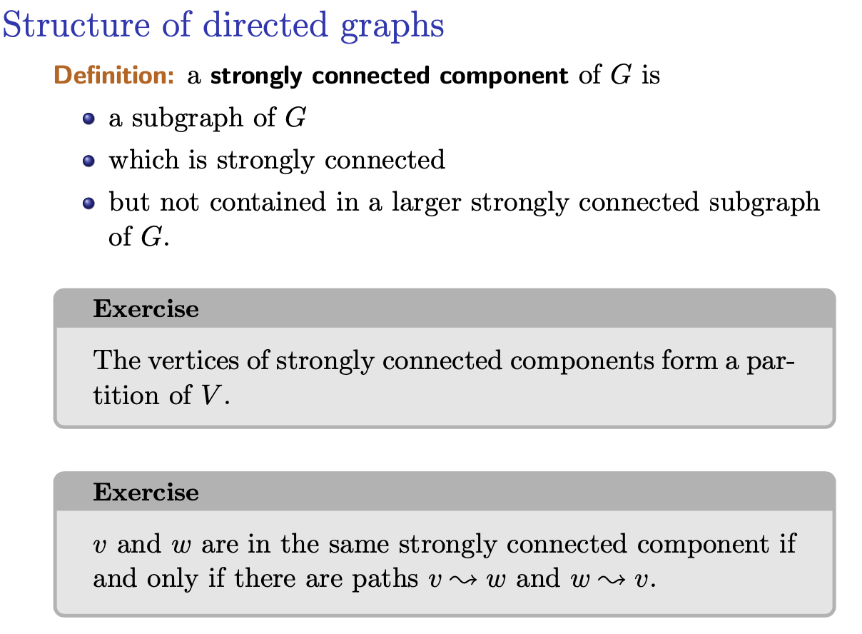
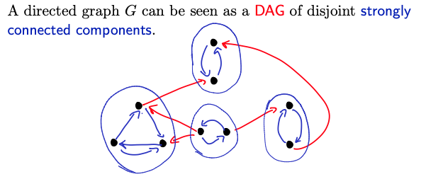
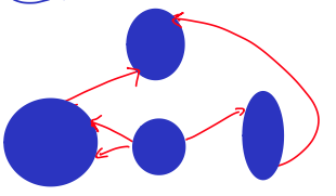
If given a directed graph we can form a strongly connected components, we can form a DAG.
Korasaju's Algorithm
Definition: for a Directed Graph , the reverse (or transpose) graph is the graph with same vertices, and reversed edges.
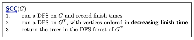
Complexity: (don’t forget the time to reverse )
Exercise: check that the strongly connected components of and are the same.
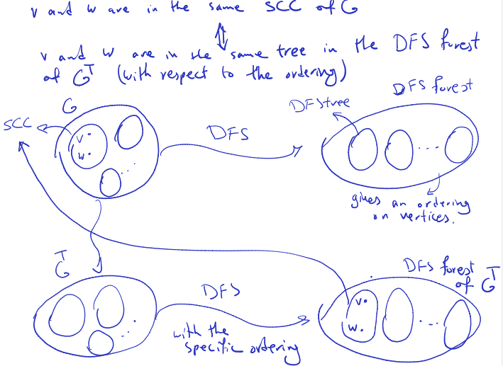
Proof: and are in the same SCC of and are in the same tree in the DFS forest of (with respect to the entering).
Run DFS in () from the node that you finished in by doing the first DFS on
Thu Feb 8 2024
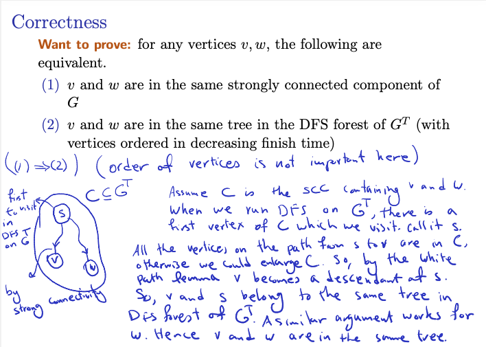
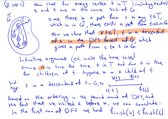
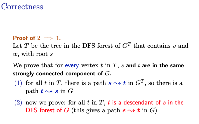
. Show that for every vertex in (including and ) and are in the same SCC of . Since there is a path from to any , which is in , there exists a path from in . Now we show that , is a descendant of in the DFS forest at , which gives a path from to in .
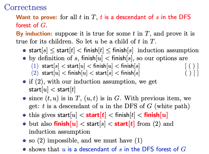
Inducting argument (write the base case). assume it is true for some in and show it is true for children of . Suppose is a child of .
Induction hypothesis: is a descendant of in , so (insert image prof drew)
Based on the ordering in the second round of DFS, and the fact that we visited before , we can calculate: …todo
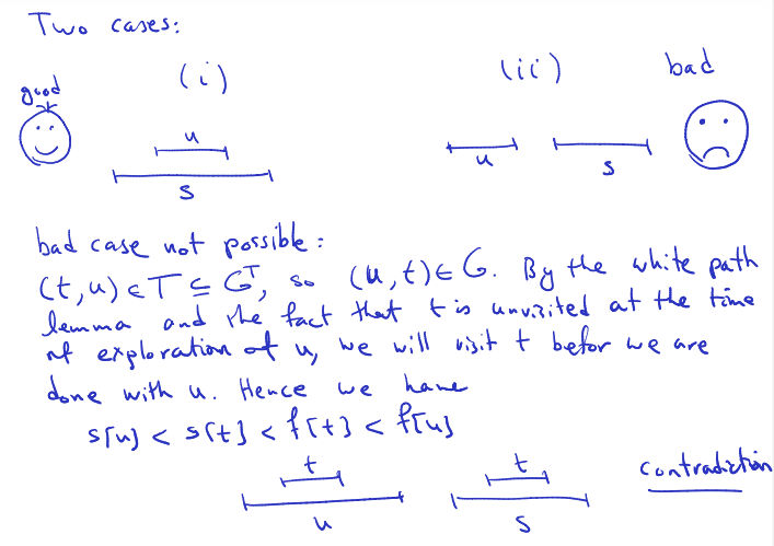
Two cases: (insert picture)
Bad case not possible: todo
Basically this slide:
True/False For a given DAG, , we have a linear time algorithm for deciding whether contains a hamiltonian path.
- can run DFS on and find a topological ordering.
- Finding a hamiltonian path is basically having a unique topological ordering
Module 4
Lecture 8 - Greedy Algorithms
Goals: This module: the greedy paradigm through examples
- interval scheduling
- interval colouring
- minimizing total completion time
- Dijsktra’s algorithm
- minimum spanning tress
Greedy Algorithms
Context: we are trying to solve a combinatorial optimization problem:
have a large, but finite, domain
want to find an element in that minimizes/maximizes a cost function
Greedy strategy:
- build step-by-step
- don’t think ahead, just try to improve as much as you can at every step
- simple algorithms
- but usually, no guarantee to get the optimal
- it is often hard to prove correctness, and easy to prove incorrectness.
Was not paying attention since rankings came out and ended talking to Chester for the whole time…
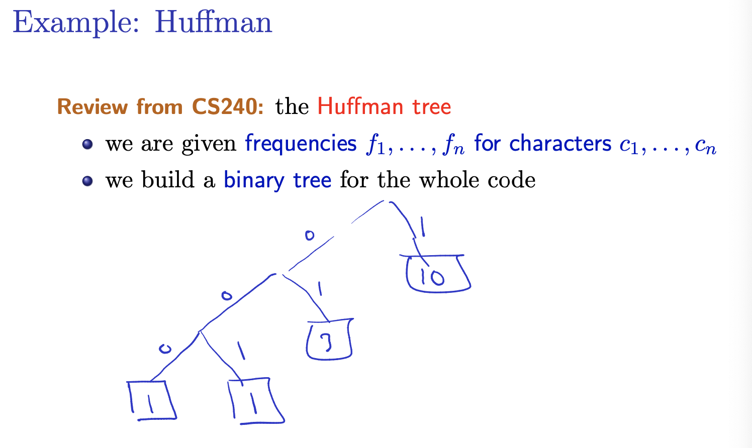
Greedy strategy: we build the tree bottom up.
- create many single-letter trees
- define the frequency of a tree as the sum of the frequencies of the letters in it
- build the final tree by putting together smaller trees: join the two trees with the least frequencies
Claim: this minimizes × {length of encoding of }
We did not look a at the Huffman Tree in CS240.
Interval Scheduling
Interval Scheduling Problem
Input: intervals . Output: a maximal subset of disjoint intervals
What does it mean?
A maximal subset of disjoint intervals refers to the largest possible collection of intervals from the given set where none of the intervals overlap with each other. In other words, you’re trying to find the largest number of intervals that can be scheduled without any conflicts in terms of time.
Example: A car rental company has the following requests for a given day
- : 2pm to 8pm
- : 3pm to 4pm
- : 5pm to 6pm Answer is
Greedy Strategies
There are different greedy strategies for solving the Interval Scheduling Problem:
- Consider earliest starting time (Choose the interval with ).
- Earliest Starting Time: This strategy selects intervals based on their starting times. It chooses the interval that starts earliest among the remaining intervals at each step. This often leads to selecting intervals that allow for the maximum number of non-overlapping intervals to be scheduled.
- Consider shortest interval (choose the interval with ).
- Shortest Interval: This strategy focuses on selecting the shortest interval among the remaining intervals at each step. By choosing shorter intervals first, it may allow for more flexibility in scheduling longer intervals later.
- Consider minimum conflicts (choose the interval that overlaps with the minimum number of other intervals).
- Minimum Conflicts: This strategy aims to minimize conflicts by selecting intervals that overlap with the fewest number of other intervals. It prioritizes intervals that have the least overlap with the currently selected intervals.
- Consider earliest finishing time (choose the interval with ).
- Earliest Finishing Time: This strategy selects intervals based on their finishing times. It chooses the interval that finishes earliest among the remaining intervals at each step. This can lead to scheduling intervals that free up resources quickly and potentially allow for more intervals to be scheduled overall.
The algorithm provided outlines a generic approach to solving the Interval Scheduling Problem using a greedy strategy based on the earliest finishing time. It sorts the intervals based on their finishing times and then iterates through them, adding intervals to the schedule if they do not conflict with previously selected intervals. Finally, it returns the selected intervals.
Algorithm: Interval Scheduling
- Sort the intervals such that
- For from to do if interval , , has no conflicts with intervals in add to
- return
Tues Feb 12 2024 (Missed class I was sleeping)
- Ask matthew for notes
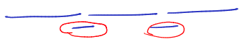
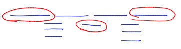
Correctness: The Greedy Algorithm Stays Ahead
Note
- is output of greedy system, is output from optimal algorithm
- If , then it must be that is optimal
- We then sort and by start/finish times
- The proof then follows:
Prof notes / proof:
- By ind. hyp.: 1.
- Compare and 2.
- 1 and 2
- At the time the greedy algorithm had to choose the interval, was an option (it had no intersection with and others). The greedy algorithm chose and it means:
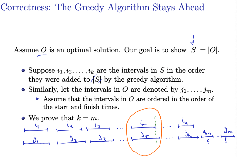
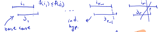
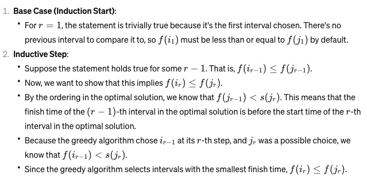
Lemma
For all indices we have .
Proof: We use induction
- For the statement is true.
- Suppose and the statement is true for . We will show that the statement is true for .
- By induction hypothesis we have .
- By the order on we have
- Hence we have
- Thus at the time the greedy algorithm chose , the interval was a possible choice.
- The greedy algorithm chooses an interval with the smallest finish time. So, .
This lemma establishes an important property:
For any index up to , where kk is the number of intervals in the greedy solution, the finish time of the interval chosen by the greedy algorithm is less than or equal to the finish time of the corresponding interval chosen by the optimal solution .
The lemma states: “For all indices , we have .”
Here, denotes the finish time of the r-th interval chosen by the greedy algorithm, and denotes the finish time of the r-th interval chosen by the optimal solution.
Note
- Recall that is the i-th index from the sorted (by start/end position) Greedy output, and is the j-th index from the sorted (by start/end position) Optimal output.
- For (base case), we know that , since for the greedy approach, we always start by taking the one that finishes earliest.
- For , we use induction, and assume that , and try proving it for .
- So, by inductive hypothesis, we have , and by comparing and , we have that . Using both of those, we get that . So, when the greedy algorithm had to choose the r-th interval, was an option (it had no intersection with and others), and thus it would have chosen that, or something better. So, .
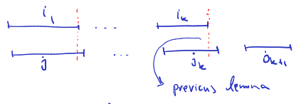
Theorem
The greedy algorithm returns an optimal solution.
Proof:
- Prove by contradiction.
- if the output is not optimal, then .
- is the last interval in and must have an interval .
- Apply the previous lemma with , and we get .
- We have .
- So, was a possible choice to add to by the greedy algorithm. This is a contradiction
Prof notes:
- Show
- Assumer . There exists at least in as it has at least one more element in comparison to .
- By the previous lemma, we know that:
- So the greedy algorithm could add to , but it did not and it is a contradiction.
Interval Colouring
Interval Colouring Problem
Input: intervals Output: use the minimum number of colours to colour the intervals, so that each interval gets one colour and two overlapping intervals get two different colours.
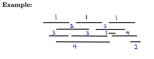
Algorithm: Interval Colouring
- Sort the intervals by starting time:
- For from 1 to do Use the minimum available colour to colour the interval . (i.e. use the minimum number to colour the interval so that it doesn’t conflict with the colours of the intervals that are already coloured.)
Note
He gives an algorithm, but he said that an one exists with a min heap and stuff, but he doesn’t care.
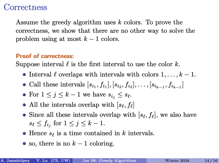
Prof’s proof:
-
If the greedy algorithm uses colours, then is the minimum number of colours needed. In other words, no other algorithm can solve the problem with colours.
-
Idea: Show that there exists a time such that it is contained in intervals.
-
Assume is the first interval which uses colour .
-
Since we have an increasing order on start times: for .
-
On the other hand all intervals have overlap with , hence for .
-
So, is the time which is contained in intervals. So, no colouring with less than colours exists.
Sanity check: Recap
This algorithm is a greedy approach to solve the Interval Colouring Problem. It sorts the intervals by their starting times and then iterate through each interval, assigning it the minimum available colour that does not conflict with the colours already assigned to overlapping intervals.
Correctness showing that if the greedy algorithm uses colours, no other way to solve problem using at most colours.
Me trying to make sense of the proof
- Suppose Intervals is the First to Use Colour :
- The proof starts by considering a interval that is the first one required colour (a new colour dumbass). This means that all previous intervals have been coloured with colours , and intervals is the first one requiring colour because it overlaps with intervals already coloured with colours .
- Interval Overlaps with Previously Coloured Intervals:
- The intervals that have been coloured with colours all overlap with interval . This means that they share some time interval with interval .
- Interval Contains Times from Intervals:
- Because all intervals have been coloured with colours overlap with interval , the start time of the interval is less than or equal to the finish time of these intervals (). This means that is a time point that is contained within intervals.
- Conclusion: No Colouring Exists:
- Because is contained within intervals, it implies that colouring interval with colour is necessary to ensure that it does not have the same colour as any of the intervals it overlaps with. If we tried to colour interval with colour or less, it would conflict with one of the intervals it overlaps with. Thus, there is no way to colour the intervals using fewer than colours while ensuring that overlapping intervals receive different colours.
Minimizing Total Completion Time
The problem
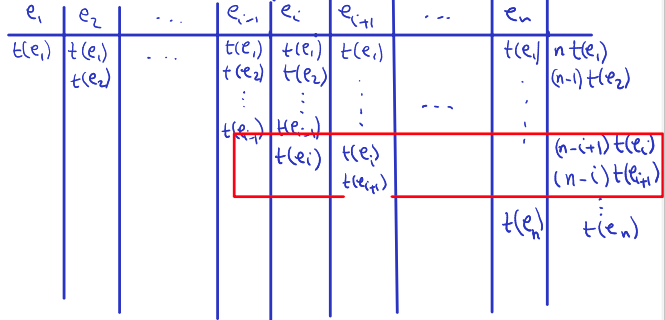
Input: jobs, each requiring processing time Output: An ordering of the jobs such that the total completion time is minimized.
Note: The completion time of a job is defined as the time when it is finished.
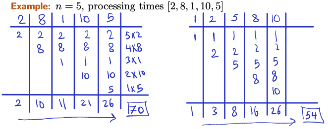
Algorithm:
- order the jobs in non-decreasing processing times
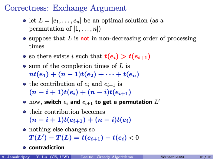
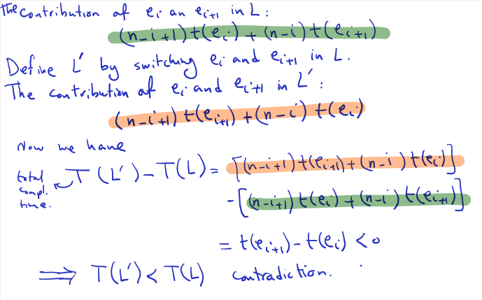
Switching position of and in the permutation , and we obtain a new permutation . And the difference in total completion time between and is calculated as: . This difference is negative because the processing time of is less than the processing time of . We have reached a contradiction which implies that by switching and we obtain a permutation with a lower total completion time than , contradicting the assumption that is an optimal solution. Therefore, the assumption that an optimal solution exists that is not in non-decreasing order of processing times leads to a contradiction, establishing the correctness of the algorithm that orders jobs in non-decreasing processing times.
Prof’s proof:
- Assume there is an optimal solution with a different ordering in comparison to the solution given by the greedy algorithm. Suppose is an optimal solution and is not in a non-decreasing order of processing times.
- So there exists an index such that the processing time of is greater than the processing time of . If this does not happen, the optimal solution has the exact same order as greedy, so if we want them to be different, it must happen.
- You can see that the cost is greater in such a case, than if you swapped and to their proper non-decreasing orders.
- So, as long as we find 1 ordering reversed, we can find something better. Thus, the optimal solution would have the ordering in non-decreasing.
Thur Feb 15 2024 (Missed class because studying for cs341 midterm)
Lecture 9 - Dijkstra’s Algorithms
Preliminaries
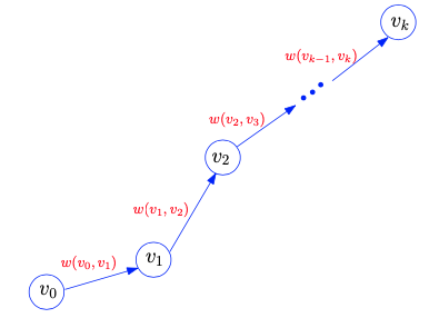
- is a directed graph with a weight function:
- Each edge has an associated weight .
- The weight of path is:
- The weight of path is the sum of weights of the edges along that path, calculated as above.
- The weight of path is the sum of weights of the edges along that path, calculated as above.
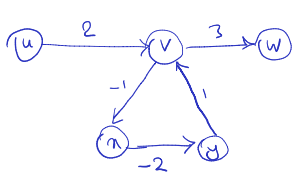
Padlet (True/False)
Shortest path exists in any directed weighted graph. https://padlet.com/arminjamshidpey/CS341
- First note that in this class, “walk vs. path” “path vs. simple path”.
- Even if there is a path between every 2 nodes, if edges can have negative weights, then it is possible that there is a cycle with negative total weight, and thus going through the cycle many times can lead to infinitely low weights. So, it is false.
- Even if there is a path between every pair of nodes, negative-weight cycles can lead to infinitely low weights by traversing the cycle multiple times.
- Negative Weights:
- When negative weights are introduced into the graph, the situation becomes more complex.
- Negative weights can lead to scenarios where paths that include negative-weight edges have shorter total weights than paths without negative-weight edges.
- This can lead to unexpected behavior, such as negative-weight cycles, where starting and ending at the same node repeatedly can result in an infinitely negative total weight.
- Impact on Shortest Path Existence:
- In graphs with negative weights, the existence of shortest paths is not guaranteed.
- Negative-weight cycles introduce ambiguity into the concept of shortest paths. If a negative-weight cycle exists, one could repeatedly traverse this cycle to achieve arbitrarily low total weights, leading to no well-defined shortest path.
- Consequently, the presence of negative-weight cycles can invalidate the concept of shortest paths in a graph.
Why Dijkstra's algorithm doesn't work with negative weights
- Dijkstra’s algorithm employs a greedy strategy, always selecting the vertex with the smallest known distance from the source vertex at each step.
- This strategy assumes that adding a new vertex to the set of vertices with known shortest distances will never result in a shorter path to any vertex than the paths already considered.
- However, in the presence of negative weights, this assumption is violated because the distance to a neighbouring vertex can decrease when traversing an edge with negative weight.
- When negative weights are present, Dijkstra’s algorithm may select a vertex based on the current shortest path information, leading to incorrect shortest path calculations.
- Negative-weight edges can create cycles where repeatedly traversing the cycle reduces the total path weight, violating the assumption made by Dijkstra’s algorithm.
- Negative-weight cycles pose a particularly challenging problem for Dijkstra’s algorithm.
- If a negative-weight cycle exists reachable from the source vertex, it can be traversed repeatedly to produce arbitrarily low total path weights, leading to no well-defined shortest path.
- Dijkstra’s algorithm, which does not account for negative weights, cannot handle this scenario and may produce incorrect results or enter into an infinite loop.
- Assumption: has no negative-weight cycles
- The shortest path weight from to :
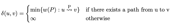
Single-Source Shortest Path Problem
Input: and a source Output: A shortest path from to each
- Aims to find the shortest path from to every other node in the graph.
- The shortest path weight from node to node , denoted as , is defined as the minimum weight among all paths from to node . If there’s no path from to , .
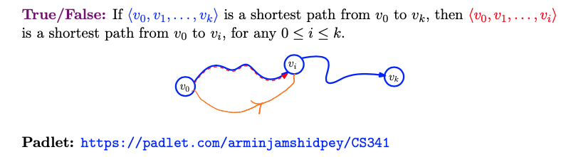
- It is true. Can prove by contradiction easily. If there was a better way, then our longer path could be shorter, which is a contradiction.
- The proof by contradiction is straightforward: Assume there exists a shorter path from to vivi for some , contradicting the assumption that is the shortest path from to .
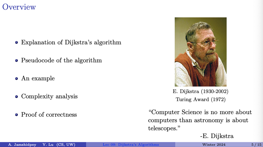
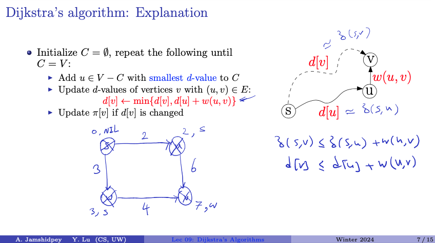
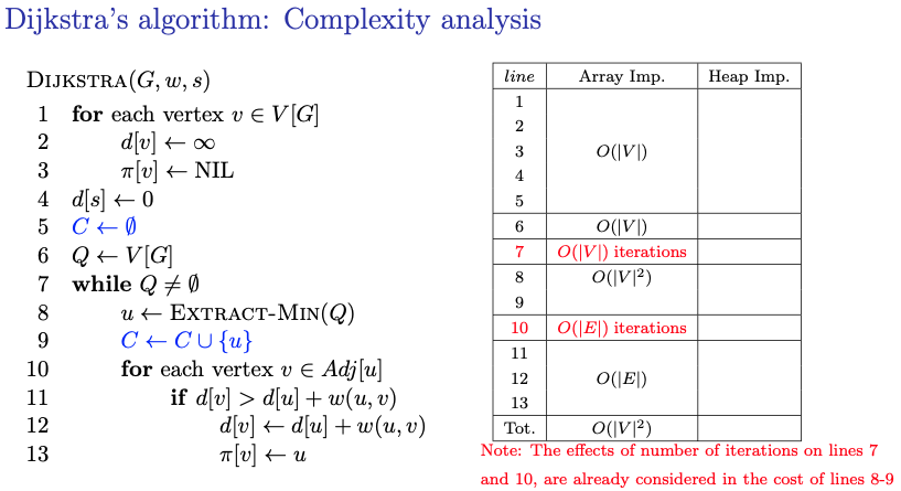
Dijkstra’s Algorithm: Explanation
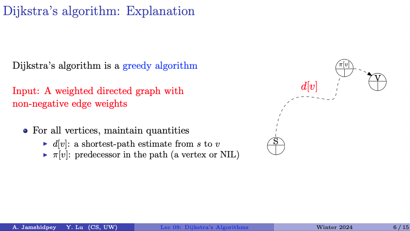
Dijsktra's algorithm is a greedy algorithm.
Input: A weighted directed graph with non-negative edge weights
- For all vertices, maintain quantities
- a shortest-path estimate from to
- predecessor in the path (a vertex or NIL)
- the predecessor in the shortest path from the source vertex to vertex .
Note:
- This is stricter than what we were saying before; not only can we not have negative weight cycles, but not even negative weight edges.
- distance level
- I think he said that refers to level
- We start by putting every parent as NIL (this is the list), and set the shortest path to infinity
- Good visualization: Dijkstra’s - Shortest Path Algorithm (SPT) Animation
- I think keeps track of vertices whose shortest paths have already been determined. So we start with being empty.
- Repeat the following steps until includes all vertices :
- Select a vertex from (i.e., the set of vertices not yet included in ) with the smallest value and add it to . This vertex becomes the next vertex to consider in the alogrithm.
- Update the of the vertices adjacent to , i.e., for each vertex such that is an edge in the graph:
- If the of any vertex changes due to the update, also update the predecessor to reflect the new shortest path.
- Termination:
- Once all vertices are included in , the algorithm terminates, and the arrays and contain the shortest-path estimates and predecessors, respectively, for each vertex from the source vertex .
I don't understand why we update predecessor
\pi[v]. I guess the question is what is the predecessor\pi[v]represent?The predecessor of a vertex in the context of Dijkstra’s algorithm represents the vertex that precedes in the shortest path from the source vertex . By updating when the -value of is changed, we ensure that always points to the vertex that is immediately before in the currently known shortest path from the source vertex . (we can use this array to reconstruct the shortest paths from the source vertex to all other vertices. starting from any , the predecessor allows us to do this.)
Which Abstract Data Type ( ADT) should we use for vertices?
Values in this tree representing a distance from a source node!
Adjacency list is my first thought
- he said no because it is a graph representation and not a vertex representation?
Prof said he would do a priority queue, which perhaps could be implemented by a min Heap.
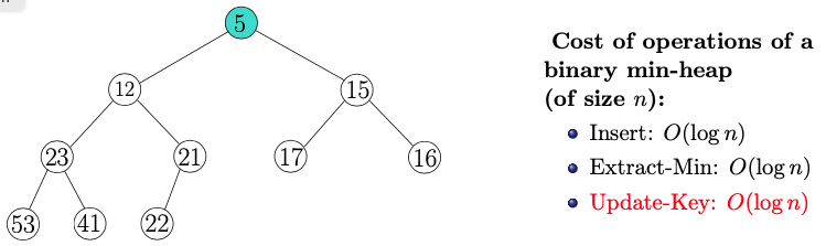
Note:
- There is the order property (left and right are larger), and the structure property (every node is full except maybe the last)
- Insert is to add a new node
- Extract-Min is to take 5 out, and fix the heap
- Apparently all the vertices are put into the min heap with values corresponding to their -value from ?
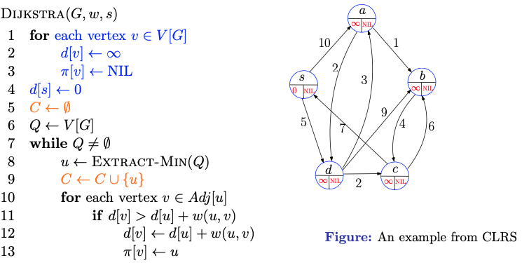
- We start by initializing everything
- The heap Q kinda keeps track of the current -values from everything.
Refer to the slides to be honest, it has a whole ass animation 20+ slides
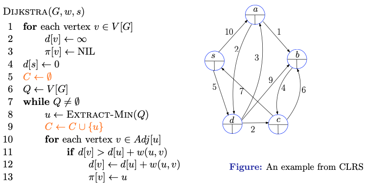
Read this part in the textbook CLRS instead.
-
Initializes the and values and empt set to keep track of vertices whose shortest paths have already been determined.
-
Initialize a priority queue containing all vertices in the graph
-
Each time through the while loop, extract a vertex from (with -value from priority queue ) and add it to set indicating that its shortest path has been determined
-
The first time through this loop . Vertex , thus, has the smallest shortest-path estimate of any vertex in .
-
For each vertex adjacent to :
- If the distance is greater than the sum of the distance and the weight of the edge from to :
- Update to , as this path is shorter
- Update to , indicating that is the new predecessor of in the shortest path from to .
- If the distance is greater than the sum of the distance and the weight of the edge from to :
-
Terminate:
- Once all vertices have been added to the set , indicating that their shortest paths have been determined, the algorithm terminates.
-
What does the orange part mean?
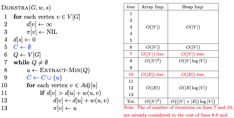
- We don’t need Heapify to make our heap because it starts with everything at
- Knowing which implementation to use depends on if the graph is sparse or not. If there are few edges (the graph is sparse), then heap is better. If there are many edges (the graph is dense), then the array implementation might be better.
Prof’s advice for the upcoming midterm tomorrow:
"It's not time for emotion, it is time for skill" - Armin
It is from michael jordan
Reading week
Ask NOTES for feb 12, 15 and 27.
Bless mattloulou
Tues Feb 27 2024 (didn’t attend class, was studying for sci250)
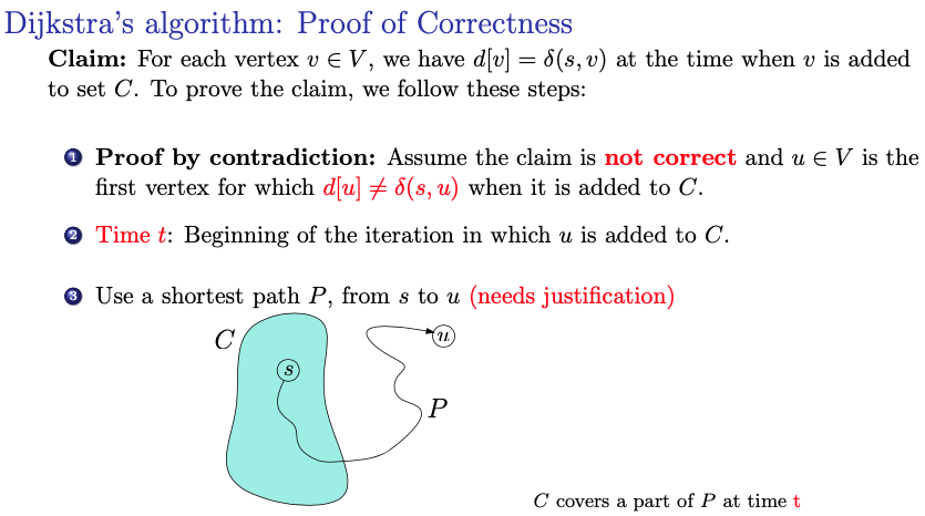 Proof:
- By contradiction: We begin by assuming that the claim is not correct, meaning there exists a vertex for which when it is added to set .
- The aim is to show that this assumption leads to a contradiction, implying that the claim must be true
- Time :
- This refers to the beginning of the iteration in which vertex is added to set .
- Shortest path :
- The existence of a shortest path from the source vertex to vertex is assumed here. This is a key assumption in the proof and must be justified.
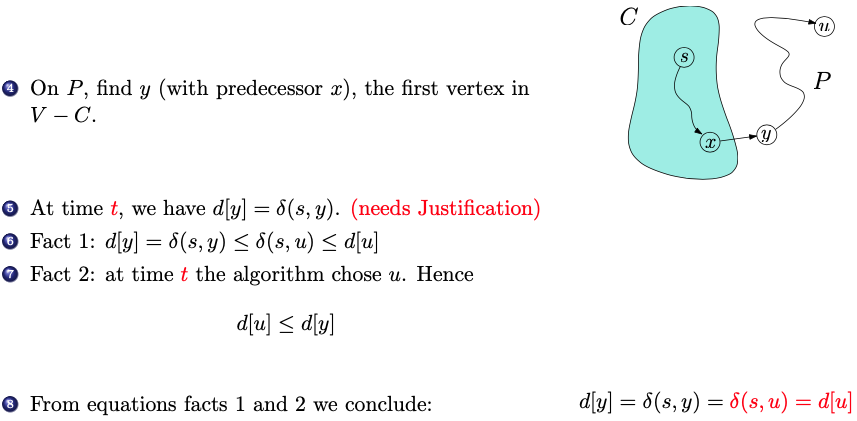
-
Finding vertex :
- On the shortest path , we find vertex as the first vertex encountered that is not already in set . This implies that is added to set after but before . (makes sense)
-
is the min weight between 2 nodes among all passes
-
The prof said that ensures that we are using non-negative weights
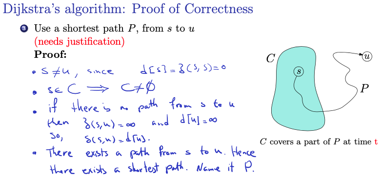
- We have that , since
- and must be distinct
- This statement ensures that the source vertex and the vertex are distinct. Which is necessary because by definition of shortest path distances.
- , so is not empty
- Since the source vertex is added to set initially, the set is not empty!
- If there is no path from to then the shortest path distance by definition and so, .
- This argument ensures that the claim holds trivially when there is no path from to .
- There exists a path from to . Hence, there exists a shortest path. Name it .
Don’t understand the last two point.
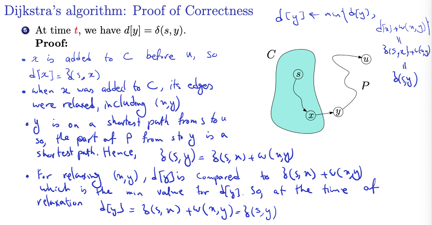
- Since is added to before , its shortest path estimate
- When was added to , its edges were relaxed, including
- What does it mean to be relaxed??? I saw it mentioned in the textbook as well
- ”Relaxation” refers to the process of updating the shortest path estimate and predecessors when a shorter path to a vertex is found during the algorithm’s execution
- When vertex is added to set , its outgoing edges, including the edge to vertex , are relaxed.
- Since is on a shortest path from to so, the part of from to is a shortest path. Hence, .
- For relaxation of edge :
- During the relaxation of edge , the algorithm compares to , which is the min value for if the path from to is indeed a shortest path.
- Since the minimum value is chosen during relaxation, at the time of relaxation
In summary
these steps provide a rigorous proof of correctness for Dijkstra’s algorithm, demonstrating that the shortest-path estimates computed by the algorithm are equal to the true shortest-path distances at the time each vertex is added to set C.
Lecture 10 - Minimum Spanning Trees
Spanning Trees
Definition:
- is a connected graph
- a spanning tree in is a tree of the form , with a subset of
- in other words: a tree with edges from that covers all vertices of the graph
- without creating any cycles
- examples: BFS tree, DFS tree
Now, suppose the edges have weights
- in many real-world scenarios, edges of a graph are associated with weights, representing costs, distances, or other measures
- each edge in the graph is assigned a weight
Goal:
- a spanning tree with minimal weight
Minimum Spanning Tree (MST):
- goal of finding a minimum spanning tree is to identify a spanning tree that includes the minimum possible total weight among all possible spanning trees of the graph.
- In other words, an MST is a spanning tree with the lowest possible total weight, considering the weights of its edges.
Note:
- This concept is particularly important in network design, where one aims to minimize costs (or maximize efficiency) while ensuring connectivity.
- This is like if you have a network and you want to minimize the cost of links, but still have everything connected, you want a minimal weight spanning tree.
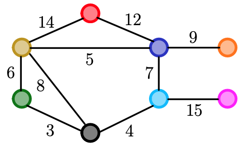
Example
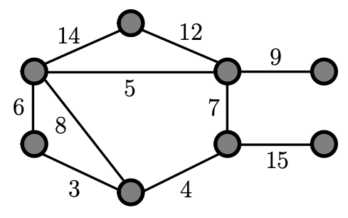
- You start off by choosing the smallest weight edges in this graph, so in the next three slides, you can see that he marked edge with weight 3, 4, 5, 6, 9 and 12, then we don’t pick 14 since we will be creating a cycle (it won’t be a minimum spanning tree)! Thus, we pick 15.
Remember the goal: We have to connect each vertices without creating any circles by choosing smaller weighting edges.
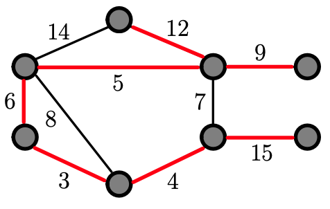
Remark: In the example, we have 8 vertices, therefore we should en up picking 7 edges, and we did. And there is no cycle and it is a tree.
Kruskal’s Algorithm
- Kruskal’s Algorithm Kruskal’s algorithm is a greedy approach to finding the minimum spanning tree (MST) of a connected, weighted graph.
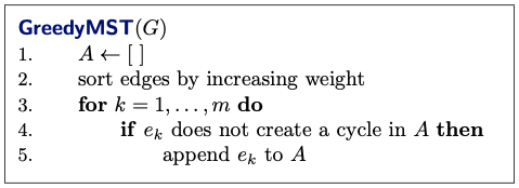
GreedyMST(G)
1. A <- []
2. sort edges by increasing weight
3. for k = 1,...,m do
4.     if e_k does not create a cycle in A then
5. append e_k to A- If there is a cycle, then it is not a tree, and so can’t be an optimal solution (assuming that edges have positive weights)
- We want to show that the result will be a tree, and so equivalently we have to show that it is connected and that there are no cycles.
Augmenting sets without cycles
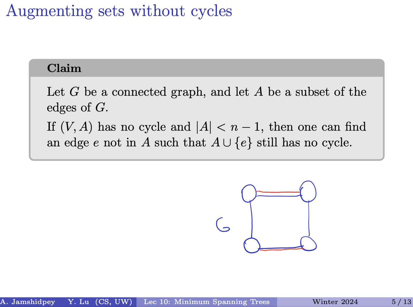
Claim
Let be a connected graph, and let be a subset of the edges of .
If has no cycle and , then one can find an edge not in such that still has no cycle.
In prof’s annotations, he proves that #vertices - #connected components #edges
- Insert Prof’s proof:
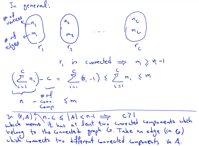
- In
- which means it has at least two connected components which belong to the connected graph . Take an edge (in ) which connects two different connected components in .
Need to understand the claim and the idea of proof.
I’m so tired right now (March 2, 2024)
Consider the connected components in the subgraph . Since , there are at least two connected components. Let’s call these connected components and .
- Each of these connected components is a subset of vertices in , and they are disconnected from each other in the subgraph .
- Since is connected, there must be at least one edge in that connects vertices from to . If there weren’t such an edge, would have been disconnected, which contradicts the fact that is connected.
- Now, let’s choose an edge from that connects a vertex from to a vertex from . Such an edge exists because is connected.
Properties of the output
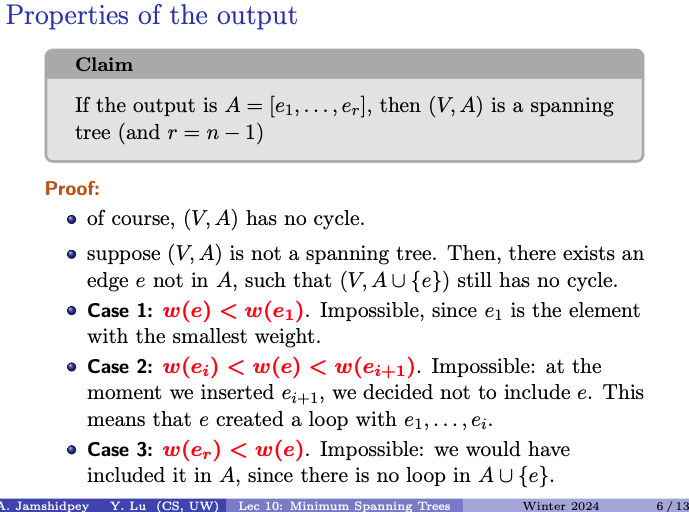
Claim
If the output is , then is a spanning tree (and ).
A spanning tree of a graph is a subgraph that is a tree (a connected acyclic graph) and includes all the vertices of .
The claim asserts that if the output of this process is a set of edges that form edges (i.e., the maximum number of edges for a spanning tree in a graph with vertices), then this set of edges indeed forms a spanning tree of the original graph .
Note: the output has edges 1 up to .
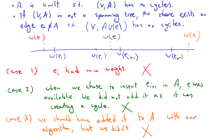
Proof:
- of course, has no cycle
- suppose is not a spanning tree. Then there exists an edge not in , such that still has no cycle.
- Case 1:
- Impossible, since is the element with the smallest weight.
- Thus, if has a smaller weight than , it should have been selected instead of . It contradicts the initial assumption.
- Case 2:
- Impossible: at the moment we inserted , we decided not to include . This means that created a loop with .
- If were to be added between and , it would create a loop with . This contradicts the fact that is assumed to be a spanning tree, which by definition is acyclic
- Case 3:
- Impossible: we would have included it in , since there is no loop in .
- If adding does not create a loop in , then it would have been included in in the first place. Since there is no loop in , it means that adding maintains the acyclic property of the subgraph, which contradicts the assumption that was no initially included in .
- These cases show that if is not a spanning tree, then there exists no edge that can be added to without creating a cycle, which contradicts the assumption that is not a spanning tree. Thus, must be a spanning tree.
Prof’s annotations:
Exchanging edges
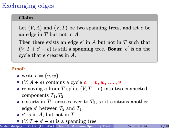
Claim
Let and be two spanning trees, and let be an edge in but not in .
Then there exists an edge in but not in such that is still a spanning tree. Bonus: is on the cycle that creates in .
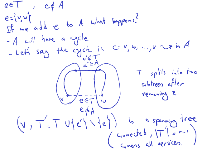
Proof:
- write
- contains a cycle
- removing from splits into two connected components
- starts in , crosses over to , so it contains another edge between and
- is in , but not in
- since c spans both and , it must contain another edge connecting and . This edge is in (since it’s part of the cycle ) but not in .
- is a spanning tree
- By replacing in with , the resulting graph remains connected and acyclic, and thus forms a spanning tree.
This completes the proof that for any edge in but not in , there exists an edge in but not in such that replacing with still results in a spanning tree.
Prof’s annotations:
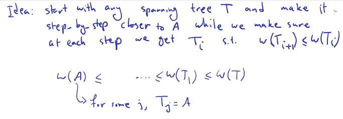
Correctness: exchange argument
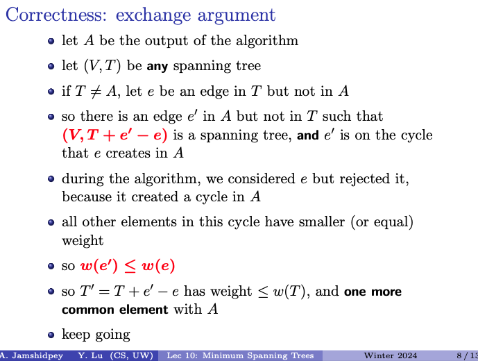
- Initial Assumption: Let be the output of the algorithm and be any spanning tree. If is not equal to , meaning there exists an edge in but not in .
- Edge Exchange: Since is in but not in , according to the claim, there must exist an edge in but not in such that replacing with results in a spanning tree .
- Weight Comparison: The claim states that is on the cycle that creates in , and during the algorithm, was considered but rejected because it created a cycle in . Moreover, all other elements in this cycle have smaller or equal weight compared to .
- Weight Inequality: Therefore, , indicating that the weight of is less than or equal to the weight of .
- Spanning Tree Construction: By replacing with , the resulting spanning tree has weight less than or equal to and one more common element with , thus maintaining the validity of the spanning tree while improving its similarity to .
- Iteration: This process can be iterated until becomes equal to , ensuring that the output of the algorithm is indeed a spanning tree similar to in terms of contained edges.
Merging connected sets of vertices
There is a slideshow of this in the notes:
…
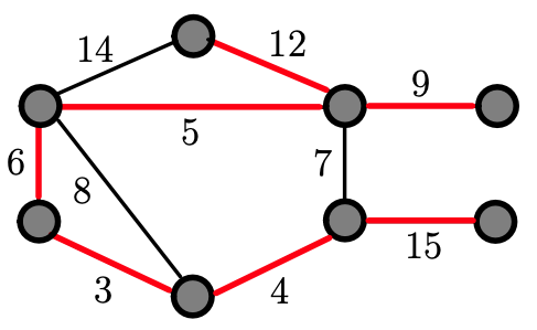
Doesn’t choose 7 because it will form a cycle. Doesn’t choose 14 because we already have all edges and by picking edge with weight 12.
Data Structures
Operations on disjoint sets of vertices:
- Find: identify which set contains a given vertex
- Union: replace two sets by their union
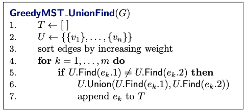
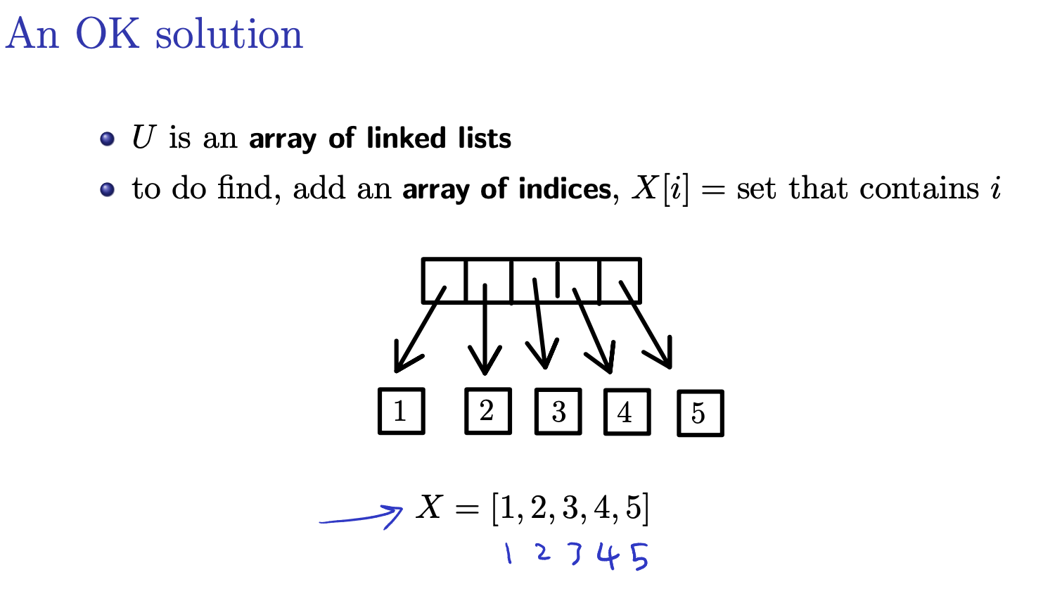
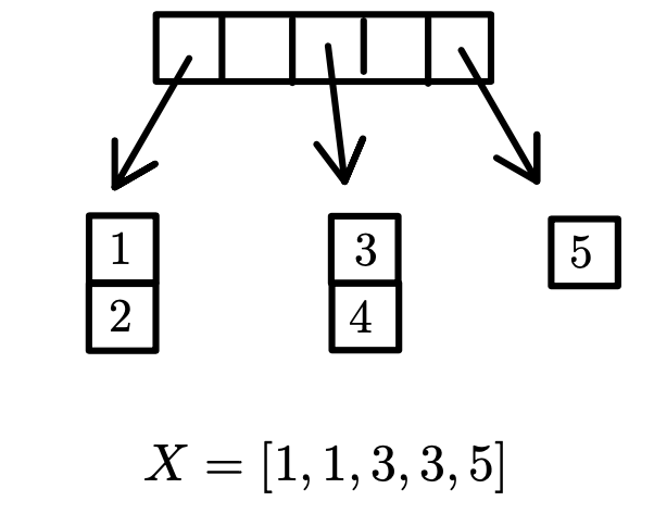
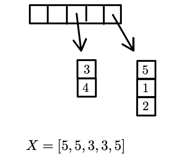
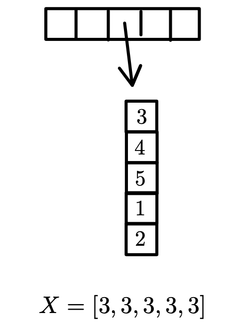
This pseudocode outlines the implementation of Kruskal’s algorithm for finding the Minimum Spanning Tree (MST) of a graph using disjoint sets (also known as Union-Find data structure).
- Initialization: Initialize an empty set to store the edges of the MST, and initialize a set containing disjoint sets, each representing a single vertex of the graph.
- Sort Edges: Sort the edges of the graph by increasing weight. This step ensures that we process edges in non-decreasing order of weight.
- Iterate Through Edges: Iterate through the sorted edges , where is the total number of edges in the graph.
- Check Connectivity: For each edge , check whether the vertices and belong to different sets in (i.e., they are not already connected in the MST).
- Union Operation: If the vertices of are in different sets, perform the Union operation on the sets containing these vertices in the MST.
- Update MST: add the edge to the MST .
- Output MST: After processing all edges, the set contains the edges of the MST.
Another slideshow of An OK solution (look in notes):
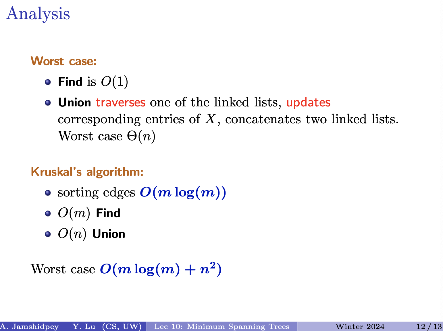
Worst case:
- Find is
- finding the set that contains a given vertex is because it simply requires a constant-time lookup in the array.
- Union traverses one of the linked lists, updates corresponding entries of , concatenates two linked lists. Worst case .
- this operation involves traversing one of the linked lists (which may contain up to elements), updating corresponding entries of , and concatenating two linked lists. In the worst case, takes time.
Krushal’s Algorithm:
- sorting edges
- using an efficient sorting algorithm
- Find
- performed for each edge to determine whether the vertices of the edge belong to different sets. Since the find operation is , total time complexity for find operations in Kruskal’s algorithm is .
- Union
- Union operations are performed whenever two vertices from different sets are found. In the provided implementation, the worst-case time complexity for a single union operation is . In Kruskal’s algorithm, there can be at most union operations (when all vertices are initially in separate sets and are merged one by one). Thus, the total time complexity for union operations in Kruskal’s algorithm is .
Worst case
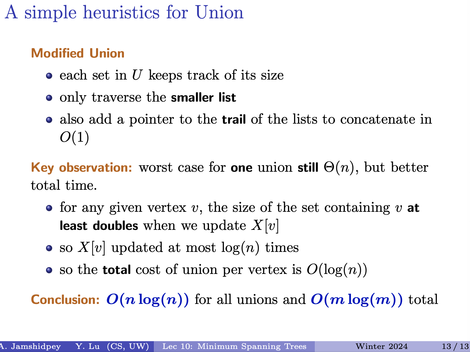
For optimizing the union operation in the disjoint set data structure which improves the overall time complexity of Kruskal’s algorithm.
- Size Tracking: Each set in now keeps track of its size. This allows us to determine which set is smaller and traverse only the smaller list during the union operation.
- Efficient Concatenation: A pointer to the tail of the lists is added to facilitate concatenation in constant time .
Analysis of Improved Version:
- Key Observation: Although the worst-case time complexity for a single union operation remains , the total time is significantly reduced due to the optimization.
- Size Doubling: For any given vertex , the size of the set containing at least doubles when we update during a union operation.
- Frequency of Updates: Since is updated at most times (as the set size doubles), the total cost of union per vertex is .
- Total Time Complexity: With the improved union operation, the total complexity for all unions becomes , considering vertices.
Combining everything: for all unions and total
Thu Feb 29 2024
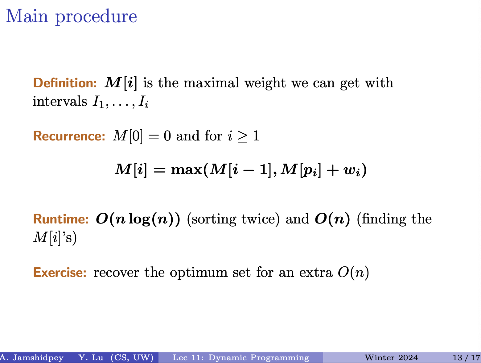
Lecture 11 - Dynamic Programming
Goals: This module: the dynamic programming paradigm through examples
- interval scheduling, longest increasing subsequence, longest common subsequence, etc.
What about the name?
- programming as in decision making
- dynamic because it sounds cool.
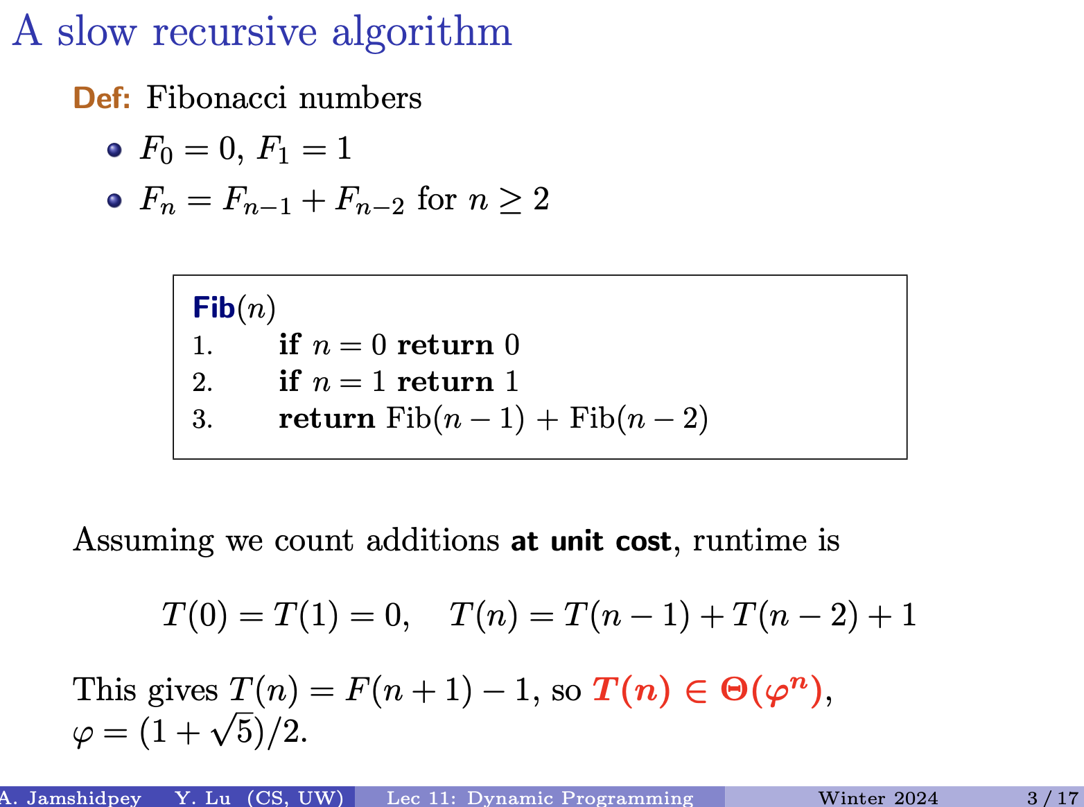
- Runtime that is exponential bigger than 1. He doesn’t look happy.
Insert picture:
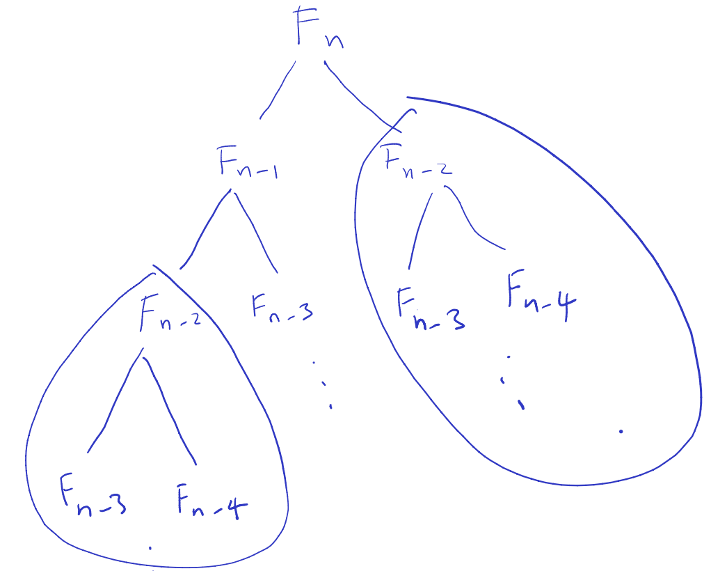
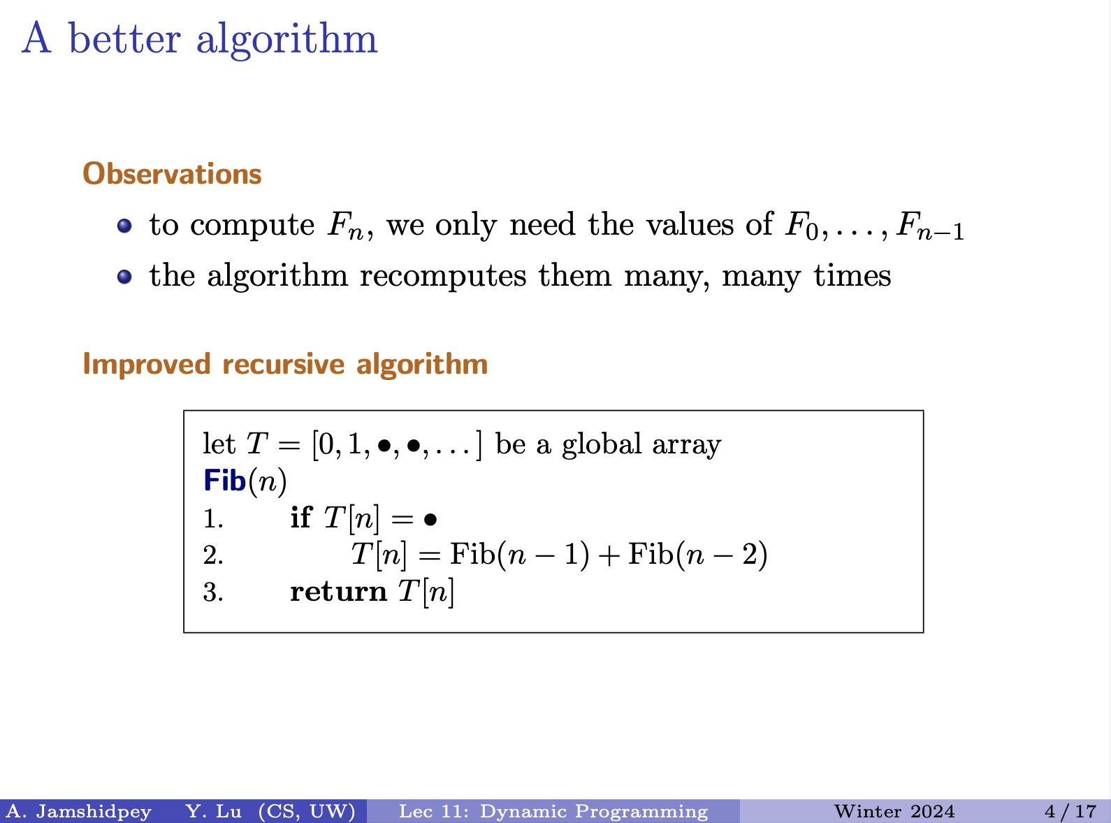
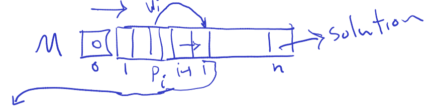
Remember what we’ve computed with an array. This is still a recursive solution. Why start by top of the tree when we can go from bottom of the tree?
Runtime:
For the data structure we will use to store , we just need an array of size (cause we start at .
- In this top-down approach, it uses the “memoization” technique, also known as “top-down dynamic programming”. Where you start by solving the larger problem by breaking it down into the subproblems. Then to avoid redundancy, you keep track of everything in a data structure, in this case an array of already computed numbers (of my subproblems).
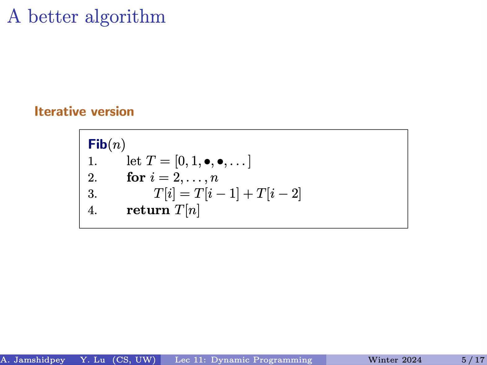
How can we improve it? Not necessarily the complexity?
We don’t care about the whole array when we only need the previous two values to compute the next.
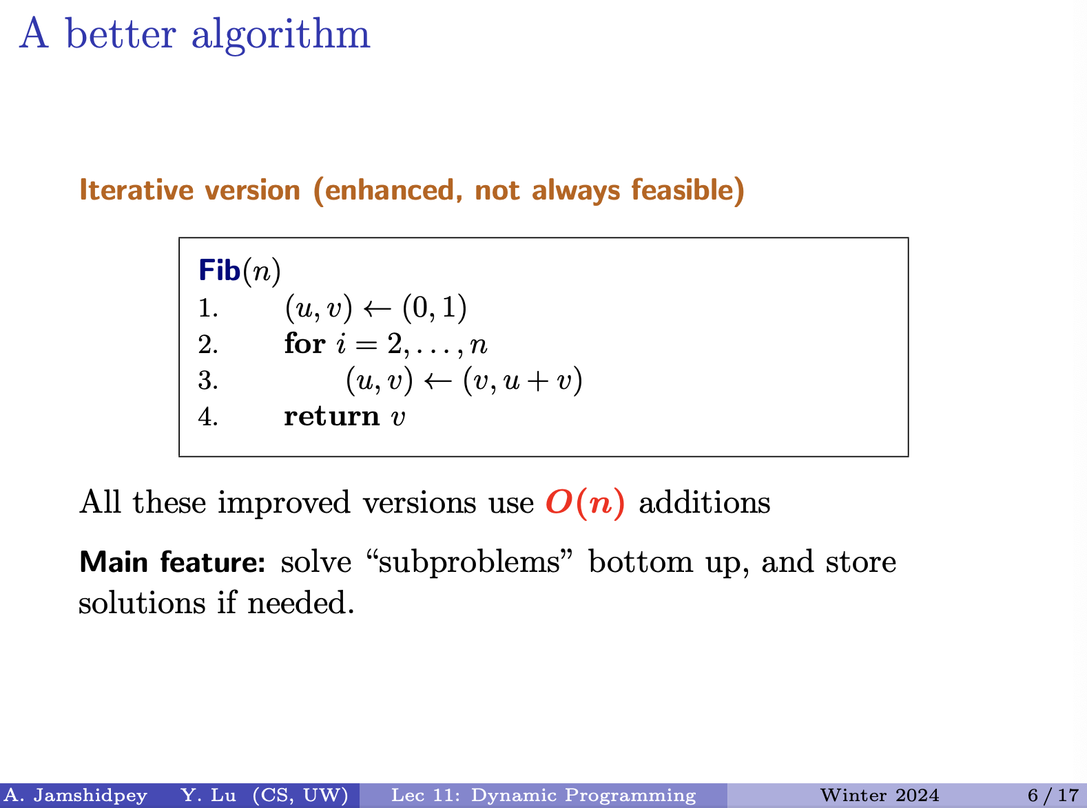
- Therefore, we have solved the subproblems from bottom up? What does that actually mean?
From chatgpt "bottom up"
In the context of dynamic programming, “bottom-up” refers to an approach where you start solving the problem from the smallest subproblems and gradually build up solutions to larger subproblems until you reach the desired solution.
In summary
- Bottom-up dynamic programming starts from the smallest subproblems and builds up solutions to larger subproblems iteratively.
- Top-down dynamic programming starts from the largest problem and breaks it down into smaller subproblems, recursively solving them while storing solutions to avoid redundant computations.
We just need an array to store stuff. No need of a hash-map. What would be the size of the array. What about ?
: so to compute the value at position we add up the values at and . What kind of relation is this?
Came up with a plan, identified the subproblems. Need a place to keep the information. Use an array, size and we know how to compute , then we tell it how to solve it.
Prof doesn’t like this slide:
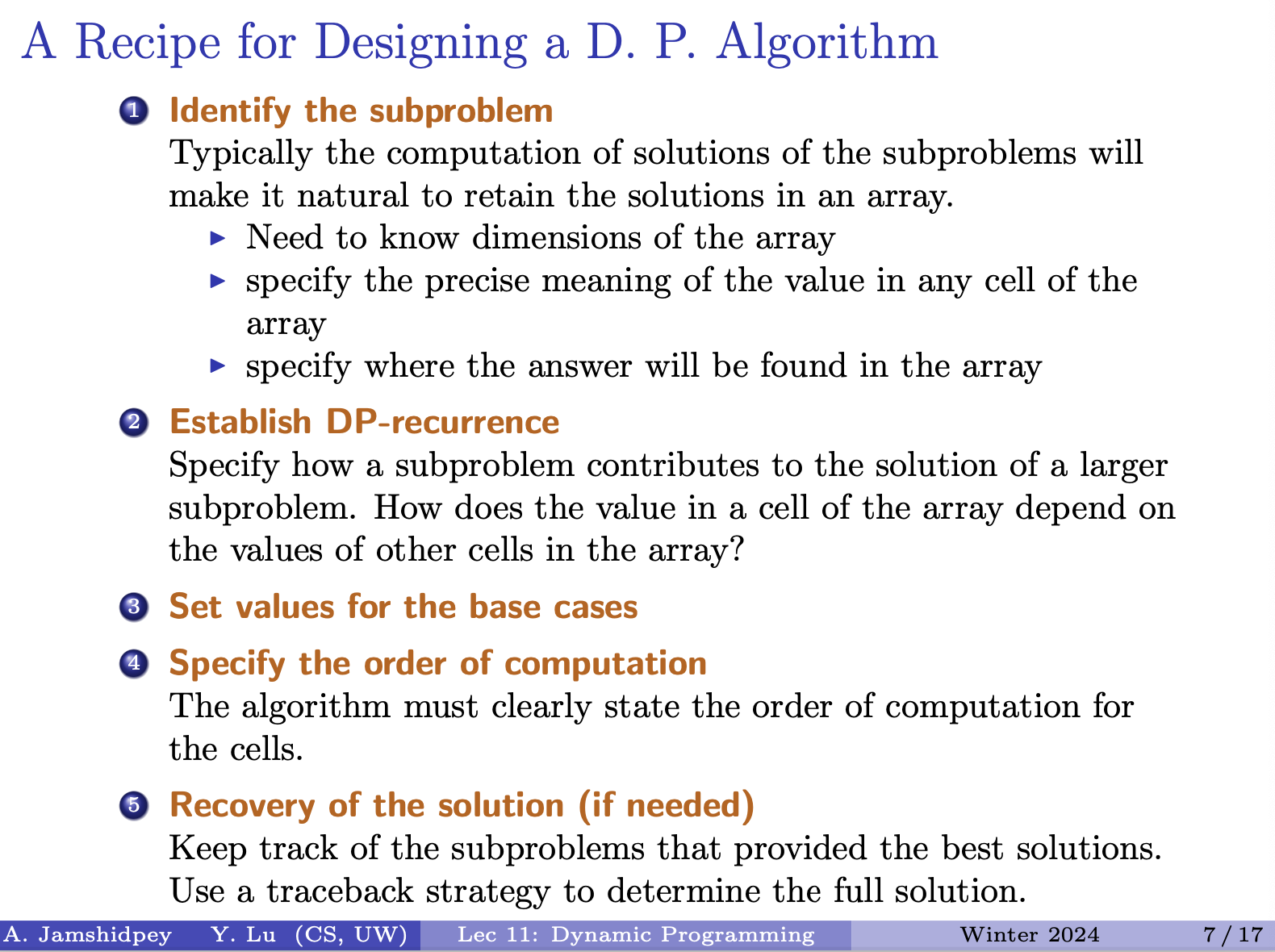
Use your creativity instead of following this recipe. - Armin
Freedom comes with a cost. Any good things come with a cost - Armin
From Matthew’s notes:
- The prof mentioned that you often might have the proof of correctness embedded into your description of the algorithm, since you often need to do a lot of justification to make the recurrence relation between your subproblems / for your algorithm to make sense.
- The prof said that in this course, point #5 is always needed. He said that in the following examples, what he is talking about will become apparent / will make sense.
- In this course, the prof said that if he asks you to do DP, you must do things iteratively, and not recursively.
Be precise on the exam, what are your subproblems, and HOW you can find the solution in the array. Then come up with a recurrence.
Recovering of the solution it is needed in this course for exams and assignments (although the slide says if needed).
In this course, when they asked dynamic programming, do it iteratively not recursively!
Dynamic Programming
Key features
- solve problems through recursion
- use a small (polynomial) number of nested subproblems
- may have to store results for all subproblems
- can often be turned into one (or more) loops
Dynamic programming vs. divide-and-conquer (PROF DOESN’T CARE ABOUT DIFFERENCES)
- dynamic programming usually deals with all input sizes
- Does not go through all the subproblems in divide-and-conquer
- DAC may not solve “subproblems”
- DAC algorithms not easy to rewrite iteratively
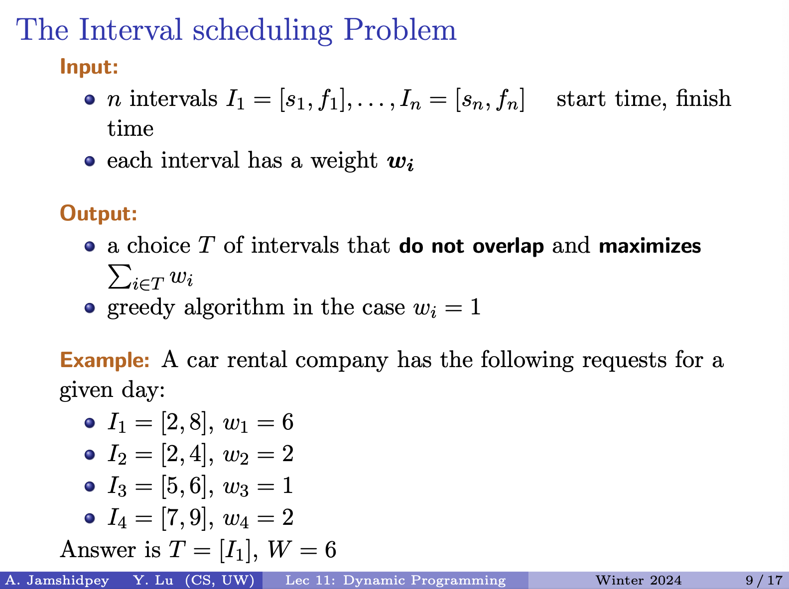
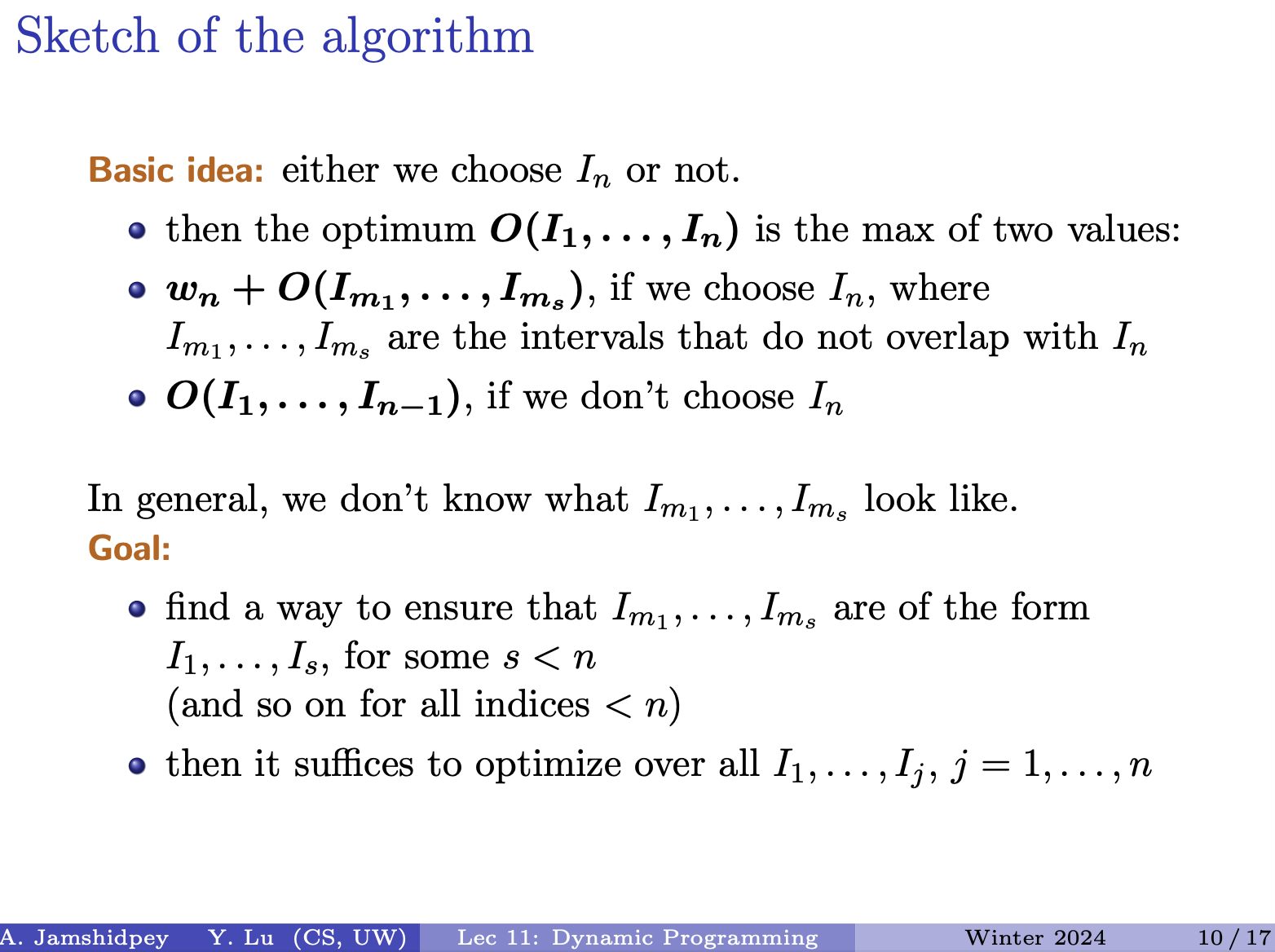
- We want the weight of the sum of the intervals to be maximized. dynamic programming solves this problem.
- We did the greedy algorithm for it before, but that only works for when the weight of each interval is 0.
- What is the input and output. Input is the number of intervals and output intervals that do not overlap and maximizes the weight.
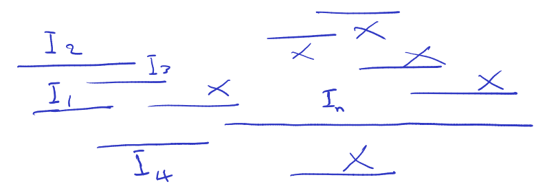
Insert picture: second is solution not containing
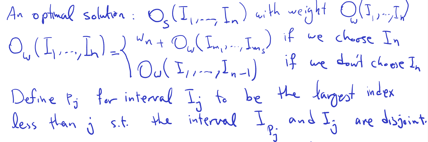
An optimal solution: with weight
- The s in the brackets which is the optimal solution, are possible candidates contributing to the optimal solution
- But we don’t know the indices of these items!
Plan to figure out the intervals that play a role in our optimal solution:
- sorting based on their finishing time. first finishing will have 1, then 2, etc.
There are two options: either we choose or we don’t choose .
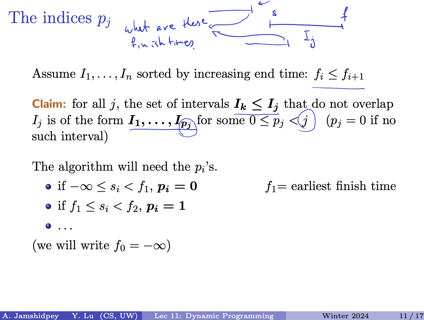
Define for interval to be the largest index less than such that the interval are disjoint. (so the next interval will have interval between those two.)to-understand
- O(…) here has nothing to do with Big-O, it is just used to show “the optimal solution that involves them”. So, the things inside the brackets are things that could be in the optimal solution, but they don’t have to be. The solution will just be a subset of them.
The idea:
- Sort the finishing time in non-decreasing order
- Initialize empty set T to store the selected intervals
- What exactly is over here?
- all the intervals that don’t overlap with the j’s Interval. Of the form
- And the ‘s? Oh maybe some sort of numbering for the intervals that belongs in between the actual Intervals depending on the finishing time of the interval. So we, that is < then . Then in this case , since it’s technically the first one.
- You somehow use to find the
- seems to be a numbering system for intervals based on their finishing times. helps in determining the index of the previous non-overlapping interval
and : represents the largest index less than such that the interval is disjoint from . This means that identifies the last interval before that doesn’t overlap with . As for , it seems to be a numbering system for intervals based on their finishing times. It helps in determining the index of the previous non-overlapping interval.
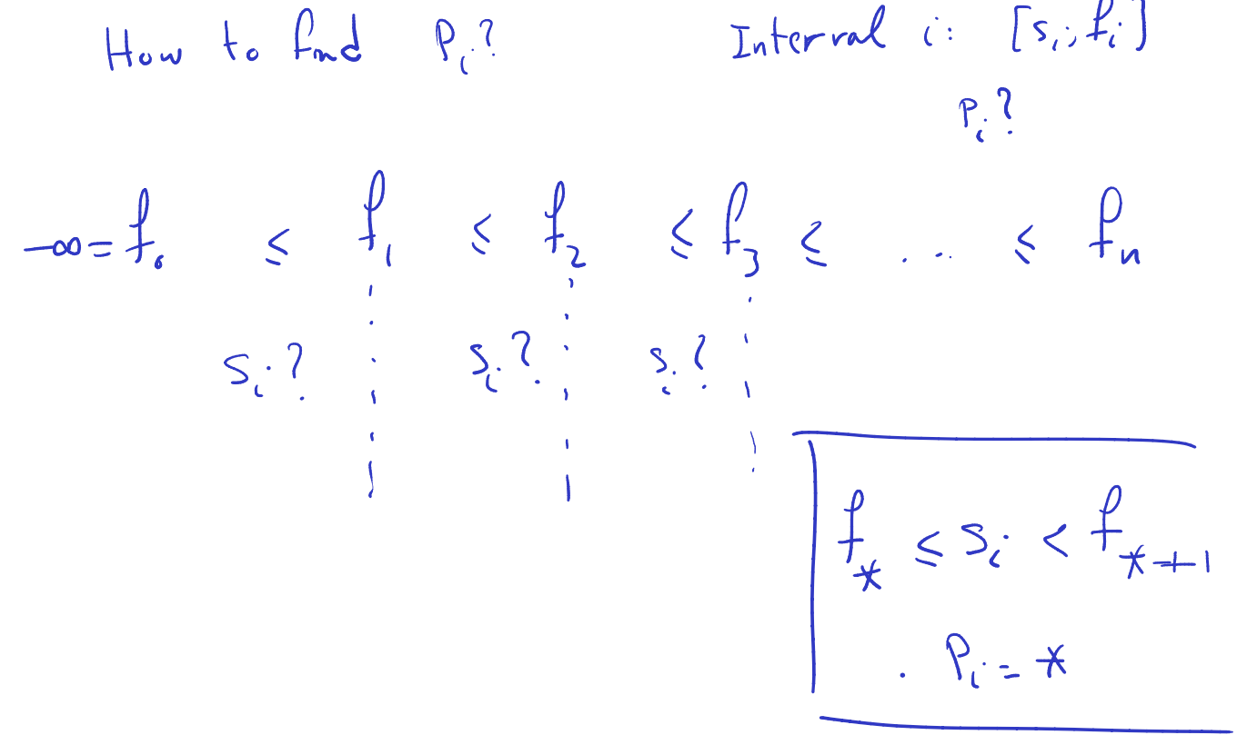
- How can I find ?
- (Interval )
- ?
- do for all the , but don’t sort because we don’t want to scramble the finish times we’ve sorted
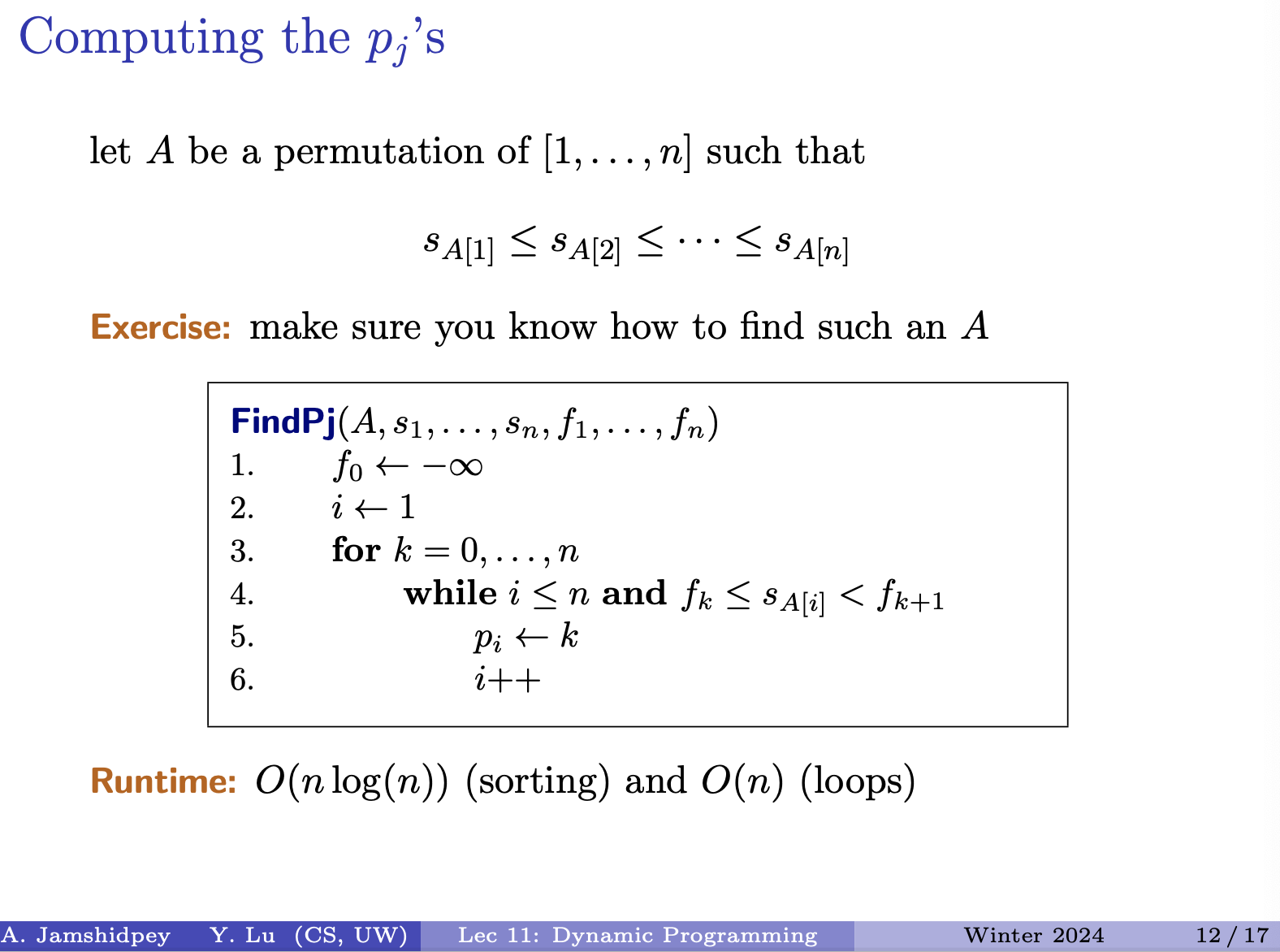
= sorting permutation for the array of s’s
- He said that finding the sorting permutation can be found in (same time as sorting)
- Go through smallest and move forward checking for the next one.
- I will never go back in computation
- refers to the indexes of
- cost: we sort once to get A, and loop cost is linear. And we are always moving forward.
Runtime: sorting and loops
The algorithm outlined is for computing the values of which represent the largest index less than such that the interval does not overlap with . Here’s a breakdown of how the algorithm works:e
- Begin by initializing to and set to 1.
- Iterate over each index from 0 to .
- While is less than or equal to and is less than or equal to (the starting time of the -th interval in the sorted order), and is strictly less than , set to and increment .
- Continue this process until either all intervals are considered or the condition is not met.
- The resulting values will indicate the largest index less than such that the intervals at those indices do not overlap with the -th interval.
The runtime of this algorithm is dominated by the sorting step, which is , and the subsequent loop, which is . Therefore, the overall runtime complexity is , which simplifies to . This makes the algorithm efficient for computing the values for the intervals.
Note: The while loop
The while loop condition in the algorithm ensures that the algorithm iterates through the intervals until it finds an interval that does not overlap with the current interval being considered. Let’s break down the condition:
while i ≤ n and fk ≤ sA[i] < fk+1
i ≤ n: This condition ensures that the algorithm does not attempt to access an index beyond the bounds of the array of intervals.
fk ≤ sA[i] < fk+1: This condition checks whether the starting time of the interval indexed byA[i]falls within the range of the current interval being considered, which is defined byfkandfk+1. If it does, then it means that the intervalA[i]overlaps with the current interval. The loop continues until an interval is found that doesn’t overlap with the current interval.The while loop condition ensures that the algorithm iterates through the intervals until it finds an interval that does not overlap with the current interval being considered (
I_k). Once such an interval is found, the algorithm assigns the appropriate value ofp_iand moves on to the next interval.
- is the last index of interval that doesn’t have intersection
- Solution is the maximum weight. That is recovering solution. Finding that set.
Matthew’s notes
- To find the optimal set, you have to first find the element in M that is maximum. Then, you have to figure out what elements actually contribute to that. To do that, you have to trace back the calculation for that index and see what contributed to it. You have to backtrack.
- The prof then ran the algorithm on a sample dataset.
- I was thinking about if it matters for this problem if we have to make start/end times distinct or not, and I think that we do not have to. There does not seem to be any part of the algorithm that will be messed up if we introduce duplicate end times or start times.
What about the recurrence?
To recover the optimum set of intervals after computing the maximal weight using dynamic programming, you can follow these steps:
- Start from the last interval and backtrack through the computed values of .
- At each step, check whether including contributes to the optimal solution. This can be determined by comparing with . If they are equal, it means was not included in the optimal solution. If is greater, it means was included.
- If was included, add it to the set of optimal intervals.
- Move to the interval and repeat the process until you reach the first interval.
- The set of intervals you collected during this process will be the optimal set.
Include picture of example: Understand it.
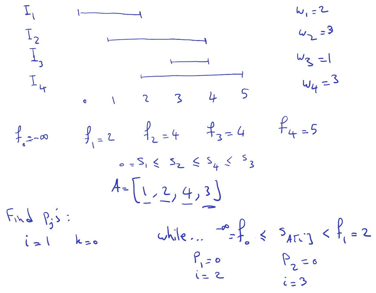
- As you can see, we first sort the intervals by their finishing time (non-decreasing order)
- Then we can find the permutation of the ‘s (But what exactly does the s represent and A)to-understand
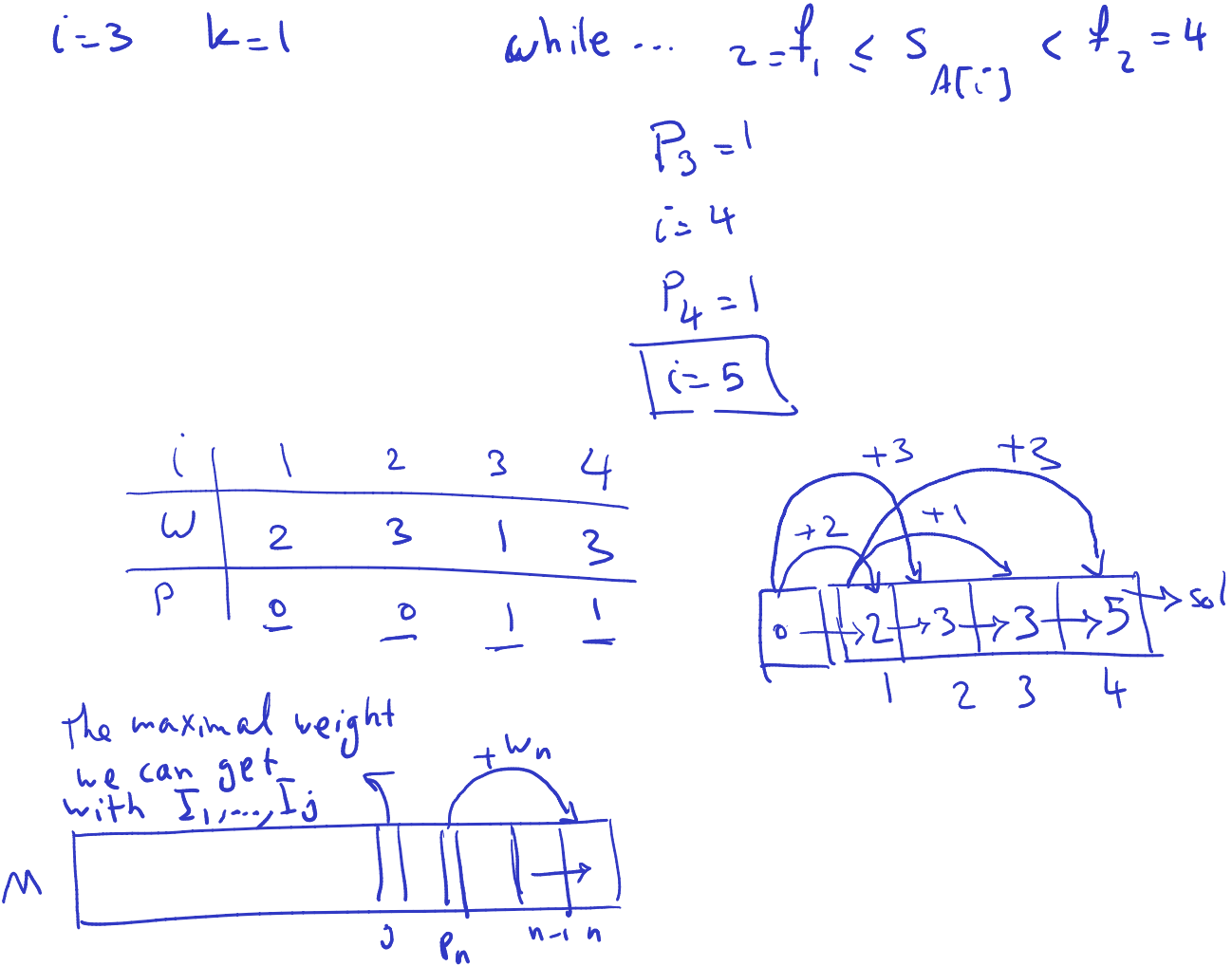
Every time you have that arrow, then this interval is in your solution. This is what you do for getting optimal solution. This is called backtracking. Basically how did we get there.
Tue Mar 5, 20204: I have recordings
Continue on slide 14/17
The 0/1 Knapsack Problem
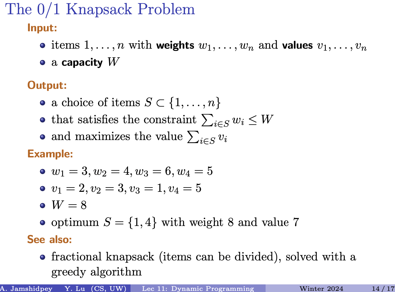
- We want to respect the weight constraint of the chosen items by optimizing the number of elements we put in.
- Does this have the constraint of only being able to pick an item once?
- In Fractional Knapsack, we can break items for maximizing the total value of the knapsack.
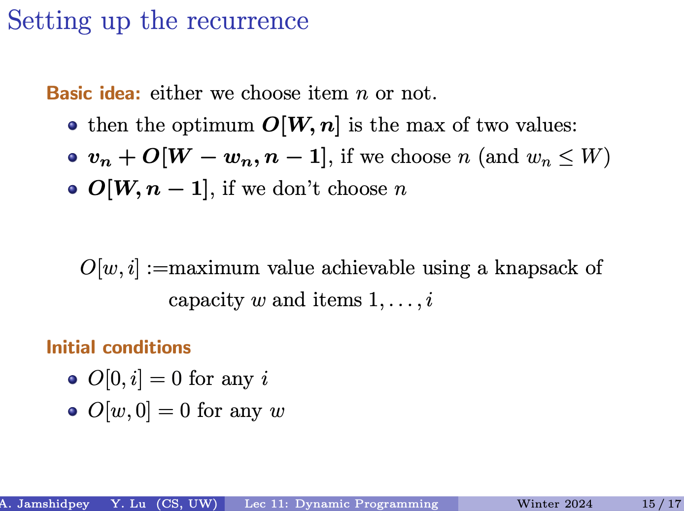
- Slide says that the optimal solution given a and items denoted as (do not confuse it with big-Oh) is the max of two values:
- , if we choose (and )
- when it says choose , i think it basically means we go through the list of the item and decide if we choose the item we are currently looking at?
- therefore we subtract that chosen weight from the upper bound
- I just don’t really understand the yetto-understand
- , if we don’t chose
- so we don’t subtract , and move on
- , if we choose (and )
- he’s’ trying to focus on one object and get the maximal value for that object
The basic idea, as you correctly mentioned, is to consider whether to include the -th item in the knapsack or not. Here’s how the recurrence relation is set up:
- If we choose to include item in the knapsack, then the value of the knapsack would be the value of the -th item plus the optimal value achievable with the remaining capacity and considering only the first items. This is represented as , where is the weight of the -th item.
- If we choose not to include item ii in the knapsack, then the value of the knapsack remains the same as the optimal value achievable using the same capacity but considering only the first items. This is represented as .
The recurrence relation can be expressed as follows:
This equation represents the optimal value function . It calculates the maximum value achievable with a knapsack of capacity ww considering items through , either by including the -th item or by excluding it.
Algorithm
Prof’s notes:
- Either we choose item a or not: The max value with items to .
- Two options:
-
- If we choose item
-
- If item is not chosen
-
- max value that we can get with weight and items to
- max value that we can get with weight and items 1 to
Insert graph: he finds items 1 at and item 2. with
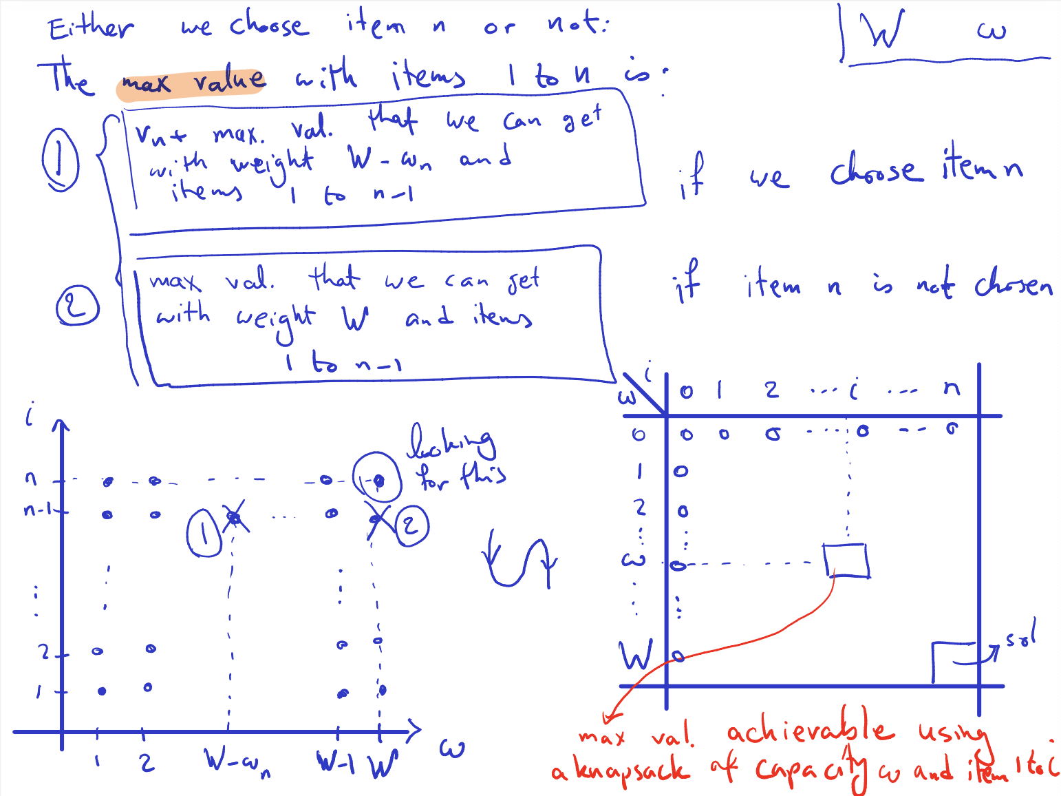
Another graph (Basically just the bottom right graph of above picture): Need to tell me precisely what are the subproblems, trying to solve problem with 1 to with capacity . You are given a and that is.
- What else does he need to give us for dynamic programming to solve
- base case
- First row, can’t add anything so all 0’s
- First column too is all of 0’s
- Order of computation:
- Take items 1 to and capacity osi , whether take item or not
- If we don’t take we have 1 to with , we can copy the cell to the cell at with capacity that is if we don’t choose the cell at with +
- Two options either take item i or not, if we take we already have in your pocket
One more thing we should be worried about. We take the best value out of the two. But is it good to take option or not. First, ask the question: Is it possible to take item or not?? If item is bigger than weight already, we don’t even have to consider it then.
- if it’s possible just compare them if not don’t need to
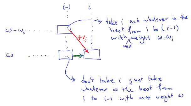
Pseudocode: Algorithm
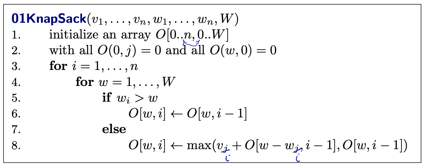
- Doesn’t show how to recover the solution in this pseudocode!
- Update maximum value: If the weight of the current item is less than or equal to the current capacity, we have two choices: either include the current item or exclude it. We choose the option that maximizes the value. The maximum value achievable considering the current item is calculated as the maximum of two values:
- : Value of the current item plus the maximum value achievable with the remaining capacity and considering only the items up to .
- : current value of item , that we are considering including or not.
- : represents the maximum value achievable with the remaining capacity and considering only the items up to -th item. It’s the max value achievable with the remaining capacity , if we decide to include item in the knapsack. We consider only the items from the first to the -th item because we have already made a decision about including item . We cannot include the same item more than once in the 0/1 Knapsack Problem, so we only consider the items before .
- Putting these two terms together, represents the total value achieved by including item in the knapsack. It adds the value of item to the maximum value achievable with the remaining capacity if item is included.
- We compare this value with the maximum value achievable without including item , which is . We choose the maximum of these two values, as it represents the optimal decision for including or excluding item in the knapsack.
- : Maximum value achievable without including the current item.
- : Value of the current item plus the maximum value achievable with the remaining capacity and considering only the items up to .
Runtime:
- Something is hidden?
- What is the actual input size? Roughly what are the parameters of the input size? Twice of so and we also have for each of those numbers: . And also is given. It is an integer. How many bits you need to store in memory. = . Is written in terms of input size. NO. Let’s rewrite it in a way we can see the input size: .
Prof’s notes:
- 0/1 Knapsack example:
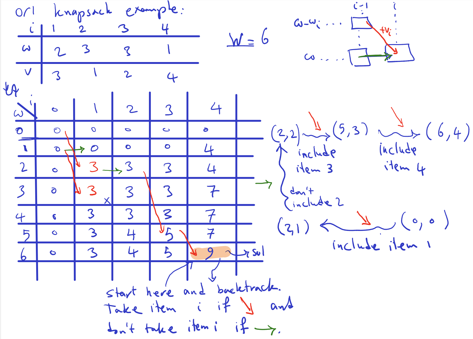
- Base case is first row and column being 0.
- Order of computation: go column by column (make sure to write the order of computation and not just draw arrows on the final exam) since in the pseudo code the outer for loop is .
- So check first if we can, if so, then look to the left and also the cell of the row - the value. and whatever in the cell + value?
- Flag those places in is taken or not: if not taken: taken from left, if taken, then the diagonal is taken.
From what I understand:
- Initialize the array: Create a 2D array
Owith dimensions(n+1) x (W+1)to store the maximum value achievable for different subproblems.O[0..n, 0..W]is initialized with allO(0, j) = 0and allO(w, 0) = 0to set the base cases.
- Iterate over items and capacities: Loop through each item
ifrom1tonand each capacitywfrom1toW. - Check if the current item can be accommodated: If the weight of the current item
wiis greater than the current capacityw, it means the item cannot be included in the knapsack. In this case, setO[w, i]equal toO[w, i-1], meaning the maximum value achievable for the current capacity without considering the current item. - Consider including the current item: If the weight of the current item is less than or equal to the current capacity, we have two choices:
- Include the current item: Add its value
vito the maximum value achievable for the remaining capacity(w-wi)and considering the previous items(i-1). This is represented byvj + O[w-wj, i-1]. - Exclude the current item: Keep the maximum value achievable without considering the current item, which is
O[w, i-1].
- Include the current item: Add its value
- Update the maximum value: Set
O[w, i]to the maximum of the two choices mentioned above. - Return the maximum value: Once the loop completes, the maximum value achievable with the given capacity and items will be stored in
O[W, n]. - Construct the solution: You can backtrack through the array
Oto find which items were included in the optimal solution. This can be done by tracing back the choices made during the dynamic programming process.
Make sure to compute the values by yourself later!
- Watch a video on it (still a bit confused)
He’s keeping track of values in his array!!!
Discussion: This is called a pseudo-polynomial algorithm
- in our word RAM model, we have been assuming all and fit in a word
- so input size is words
- but the runtime also depends on the values of the inputs
01-knapsack is NP-Complete, we we don’t really expect to do much better.
Lecture 12 - Dynamic Programming - Part 2
The Longest Increasing Subsequence Problem
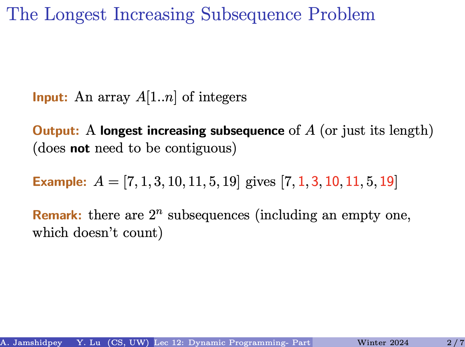
Input: An array of integers
Output: A longest increasing subsequence of (or just its length) (does NOT need to be contiguous)
Example: gives (1,3,10,11,19 red)
Remark: there are subsequences (including an empty one, which doesn’t count)
Tentative subproblems
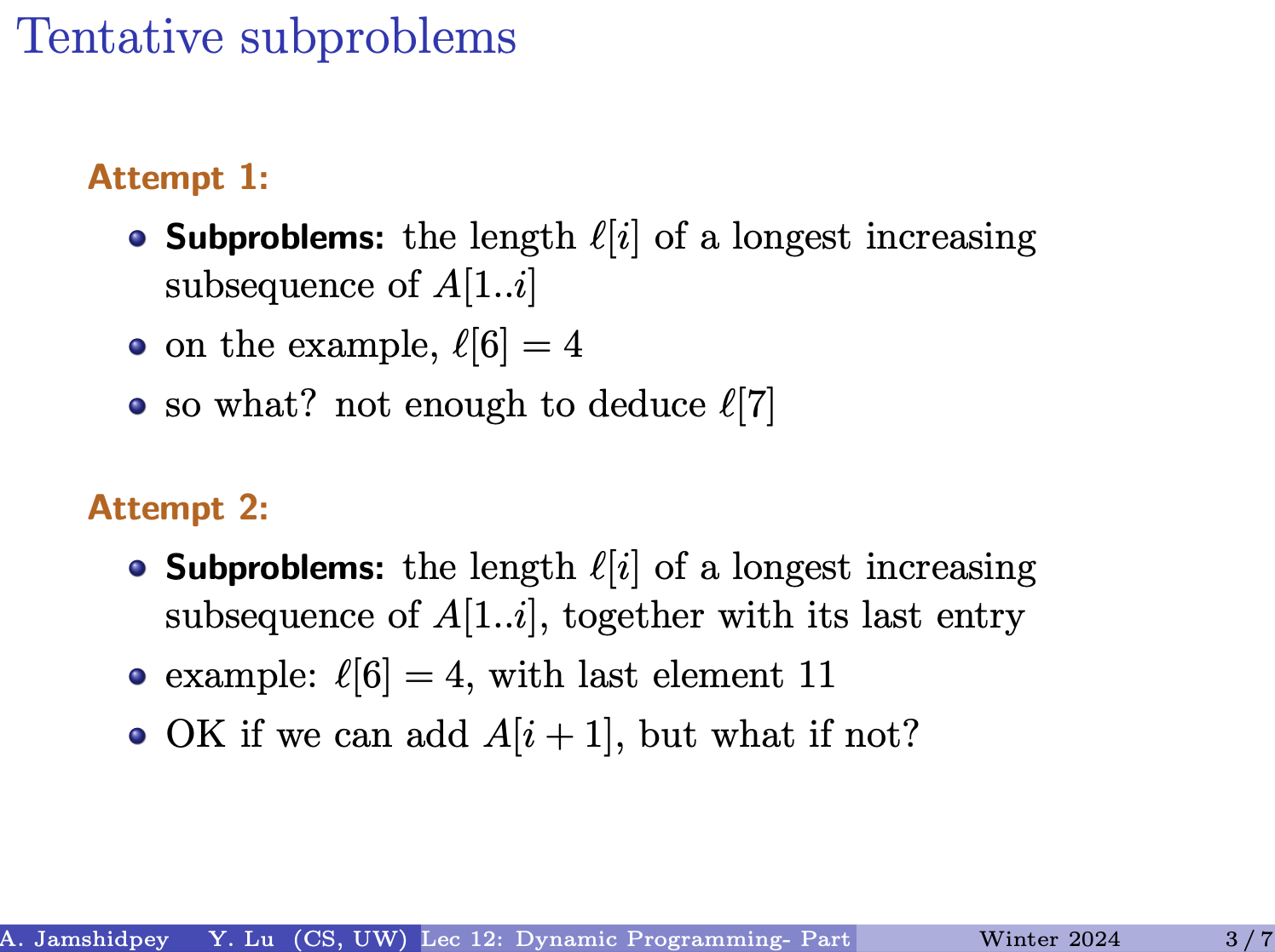
Attempt 1:
- Subproblems: the length of a longest increasing subsequence of
- \on the example,
- so what? not enough to deduce
Attempt 2:
- Subproblems: the length of a longest increasing subsequence of , together with its last entry
- example: , with last element
- OK if we can add , but what if not?
A more complicated recurrence
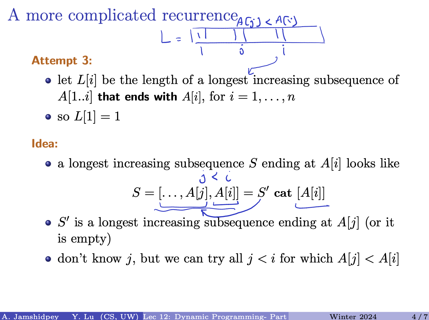
Attempt 3:
- Define as the length of the longest increasing subsequence of that ends with , for .
- Initialize , as the LIS ending at the first element is simply that element itself.
Recurrence relation:
- For each element , consider all previous elements (where ).
- If , it means can extend the LIS ending at .
- So, , where and .
Explanation:
- represents the length of the LIS ending with .
- To compute , we check all previous elements (where ).
- If , it means we can extend the LIS ending at by appending .
- We maximize this by taking the maximum of for all such .
- The final answer will be the maximum value among all .
Iterative Algorithm
When we are looking at , we don’t know where is before in the array. So we have to look at all options of and take the maximum one. So we want to keep track of . If no j, then it must be the first one?
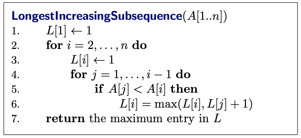
Runtime:
Remark:
- the algorithm does not return the sequence itself, but could be modified to do so
To understand
Just follow through the code with the example.
Example: Insert prof’s picture
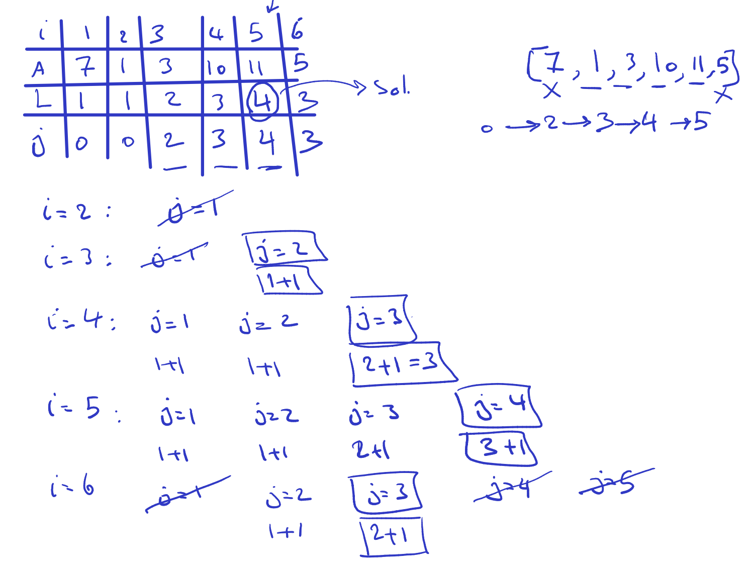
- Solution lies in array .
- how did we arrive at 5? from 4, then 3, 2 and 0. But somehow since it’s 0, we don’t take 7??
- Ok so it’s not 5 dumbass. You look at array , the highest number is 4, which is at position where 5 is in array . And you can retrace back and see that 1 2 3 4 lead to 4. So we take value in A: 1, 3, 10, 11.
Thu Mar 7, 2024: Continue and finish Lecture 12, slide 6/7
Longest Common Subsequence Problem
Longest Common Subsequence Problem
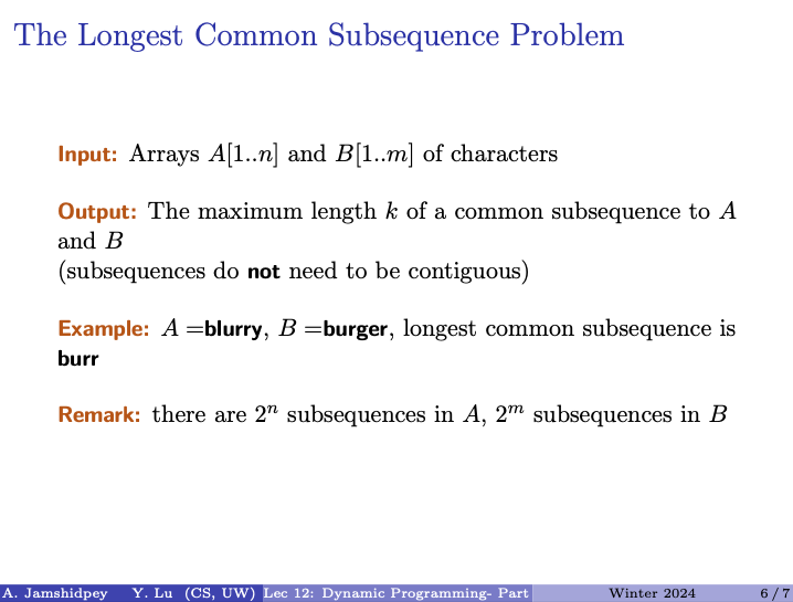
- Input: Arrays and of characters
- Output: The maximum length of a common subsequence to and . (subsequence do not need to be contiguous)
- Example: blurry, burger, longest common subsequence is burr.
- Remark: there are subsequences in , subsequences in
Prof’s notes:
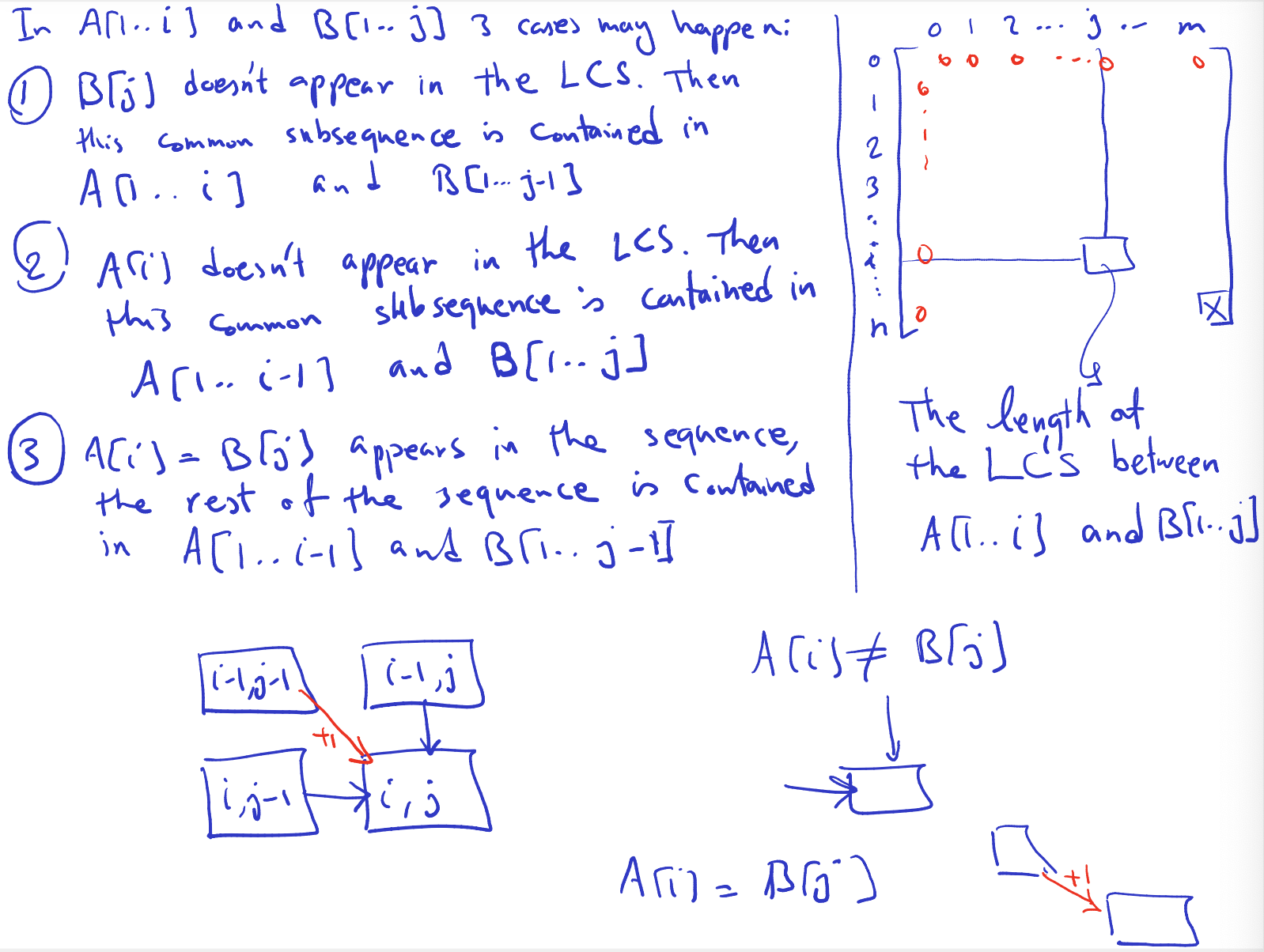
- Uses A to index his rows
- Where do i find my solution? bottom right corner.
- In and . There are 3 cases that may happen:
-
- doesn’t appear in the LCS. Then this common subsequence is contained in and
-
- doesn’t appear in the LCS. Then this common subsequence is contained in and
- The first two case are based on … not being the same
-
- appears in the sequence, the rest of the sequence is combined in and
-
Insert bottom right picture he drew:
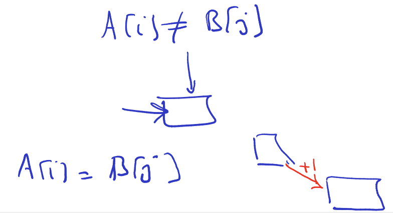
- Why add 1 in the diagonal arrow? Because They match. Dumbass.
- In the two other cases, we know we don’t have added a longest character, so don’t add one.
Approach:
- Input: Two sequences and of characters.
- Output: The maximum length of a common subsequence between and .
- Example: For example, if “blurry” and “burger”, the longest common subsequence is “burr”.
- Idea: The LCS problem can be solved using dynamic programming, typically using a two-dimensional array to store the lengths of the LCS of prefixes of the sequences.
- Recurrence: At each cell of the 2D array (where represents the index of and represents the index of ), you consider three cases:
- If , then the LCS does not include either or , so the length of the LCS up to that point remains the same as it was without including these characters. You can look at the cell or to find the length of the LCS.
- If , then you can extend the LCS by one. In this case, the length of the LCS would be one plus the length of the LCS up to the previous characters, i.e., .
- You take the maximum of these two options.
- Adding 1 in the diagonal arrow: When characters match (case 3), we add one to the LCS length because we’re extending the LCS by one character. However, in cases where characters don’t match (cases 1 and 2), we don’t add anything because the current characters don’t contribute to the LCS. So, we don’t add one in those cases.
- Finding the Solution: Once the dynamic programming table is filled, the solution lies in the bottom-right cell of the table, which represents the LCS length.
- Complexity: The time complexity of this approach is , where and are the lengths of sequences and respectively. This is because you fill a 2D array of size .
A bivariate recurrence
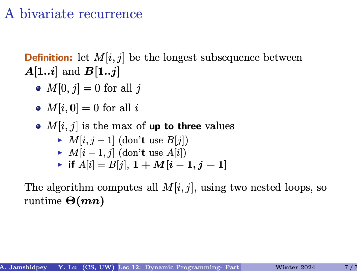
Definition: let be the longest subsequence between and
- for all
- for all
- is the max of up to three values
- (don’t use )
- (don’t use )
- if ,
Size of array is os runtime is
Prof gave an example: Insert picture
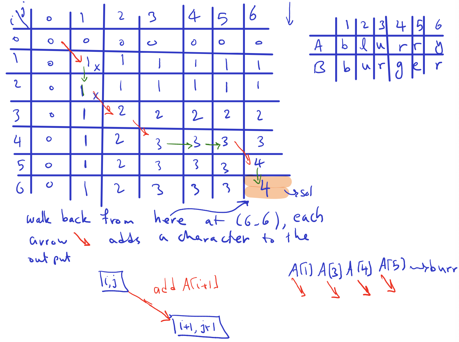
- Base case is all ‘s for first row and column
- Row is which is A. Column is which is B.
- Look if the first column is equal. they are so go diagonally. b=b
- We compare to : does not equal to . so don’t go diagonally, green arrow
- Go through the whole process by yourself at home.
- Walked through it.
- Compare (i,j)
- B, B (0,0)
- L, U (1, 1)
- U, U (2,1)
- R, R (3,2)
- R, G (4,3)
- R, E (4,4) Here instead of , we do . But why? When exactly do we advance or ????
- Y, S (5,5)
- Nothing, Y (6,5) The end.
If you want to recover your solution: Walk back from here: bottom right cell, that is in the example 4 (solution) at (6,6), each arrow (red arrow diagonal) adds a character ot the output. The first one you take is the green one, vertical. Then take the diagonal, the index of A is 5. How did i get there? diagonal red arrow. and so on
- diagonal, diagonal, diagonal, diagonal
- Note that he is not showing up every step, but when you get to your answer, you would have noted all the arrows and keep track of them. At the end, you just go back and follow them.
Insert small picture: (red arrow) add
- Can we do better? Yes, there are other heuristic, but we want talk about them. For us, the goal is to look at dynamic programming. So we don’t care. Not worried about efficiency.
When to advance or :
- When comparing characters at indices
- If equals , it means that the characters are part of the LCS. In this case, you advance both indices by diagonally to to check the next characters in both sequences.
- If does not equal , it means that the characters are not part of the LCS. In this case, you choose the maximum of the two adjacent cells????. However, you only advance one of the indices, not both.
- If you choose the maximum from the cell to the left , it means you advance index by horizontally to to check the next character in sequence .
- If you choose the maximum from the cell above , it means you advance index by vertically to to check the next character in sequence .
Should we fill up the table first then march through it?
Still not understanding the choose the max of the two adjacent cells…
I guess you need to fill up the table first. Then retrieve the answer at bottom right corner. Then backtrack from that cell to reconstruct LCS…
- Try constructing the table (used all my brain power. But definitely easier and more intuitive than 01 knapsack problem)
Dynamic Approach:
- Definition: Define as the length of the longest common subsequence between and .
- Base cases: Initialize all elements of the first row and first column of the matrix to .
- Recurrence relation: For each cell of the matrix , compute the length of the longest common subsequence using the following rules:
- If , then is the maximum of (not using ) and (not using ).
- If , then is plus (the length of LCS without the current characters plus for the match).
- Iterative computation: Use two nested loops to compute all values of . The runtime of this algorithm is , where and are the lengths of sequences and respectively.
- Reconstructing the solution: To recover the actual LCS, start from the bottom-right cell of the matrix and backtrack according to the arrows you’ve noted during computation. Follow the arrows:
- If you move diagonally (matching characters), include the character at position (or , since they are both equal).
- If you move vertically, exclude the character from sequence .
- If you move horizontally, exclude the character from sequence .
- Example: For example, if the LCS length is (bottom-right cell), backtrack from that cell following the arrows you’ve noted to reconstruct the LCS.
This approach efficiently computes the length of the LCS and allows for easy reconstruction of the LCS itself.
Lecture 13 - Dynamic Programming - Part 3
Edit Distance
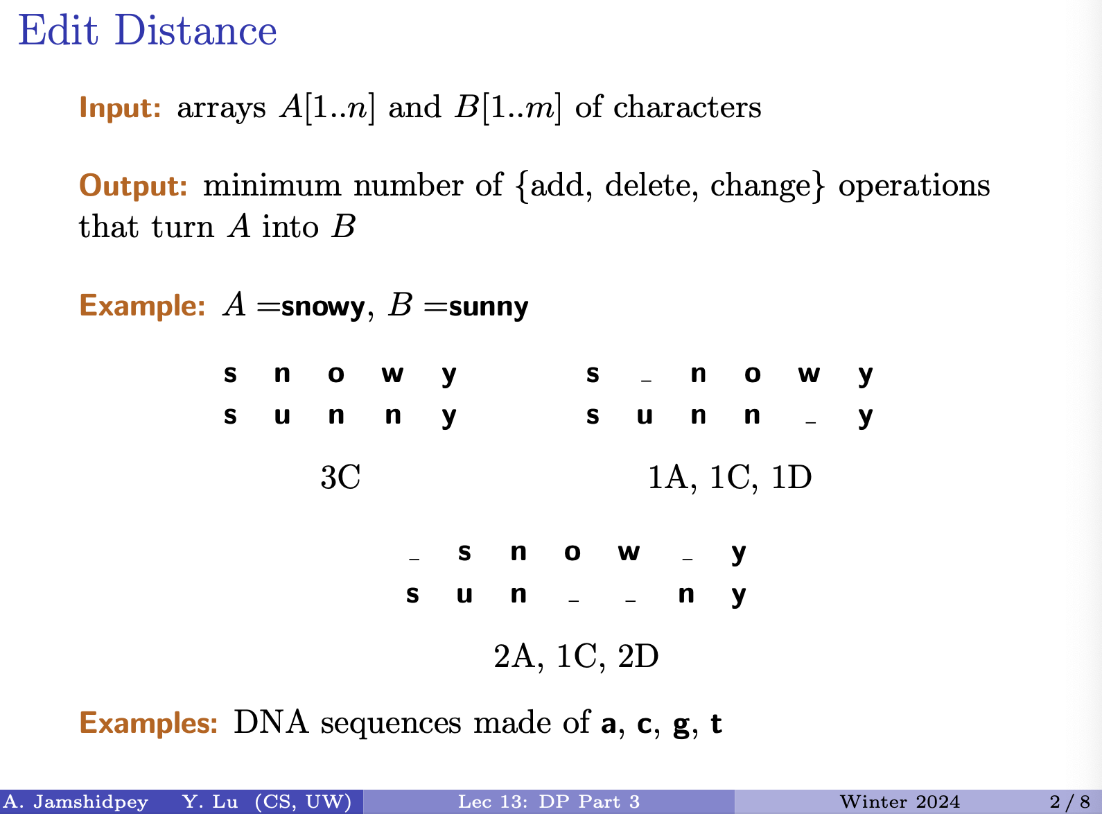
- Now here, we want to use another type of measure (he is not claiming if one measure is better than the other).
- When does mispelling happen?
-
- a character is typed wrong
- How to fix? Replace = in his slides called to fix it
-
- a character is missed
- ( to fix)
-
- An extra character is typed
- ( to fix)
-
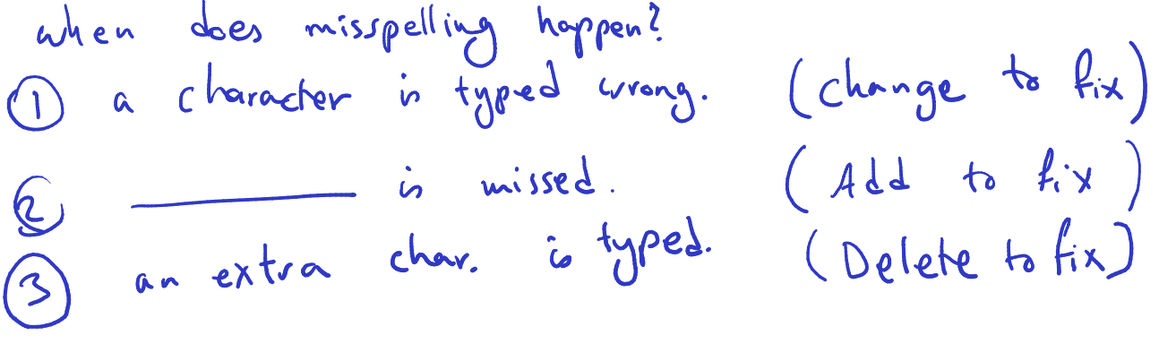
How can I convert snowy to sunny? Distance we need for editing. ED = Editing Distance
First thing to do is to align them.
- First thing is align first one
- Use a gap Out of all the alignments, you want to figure out the one that is better:
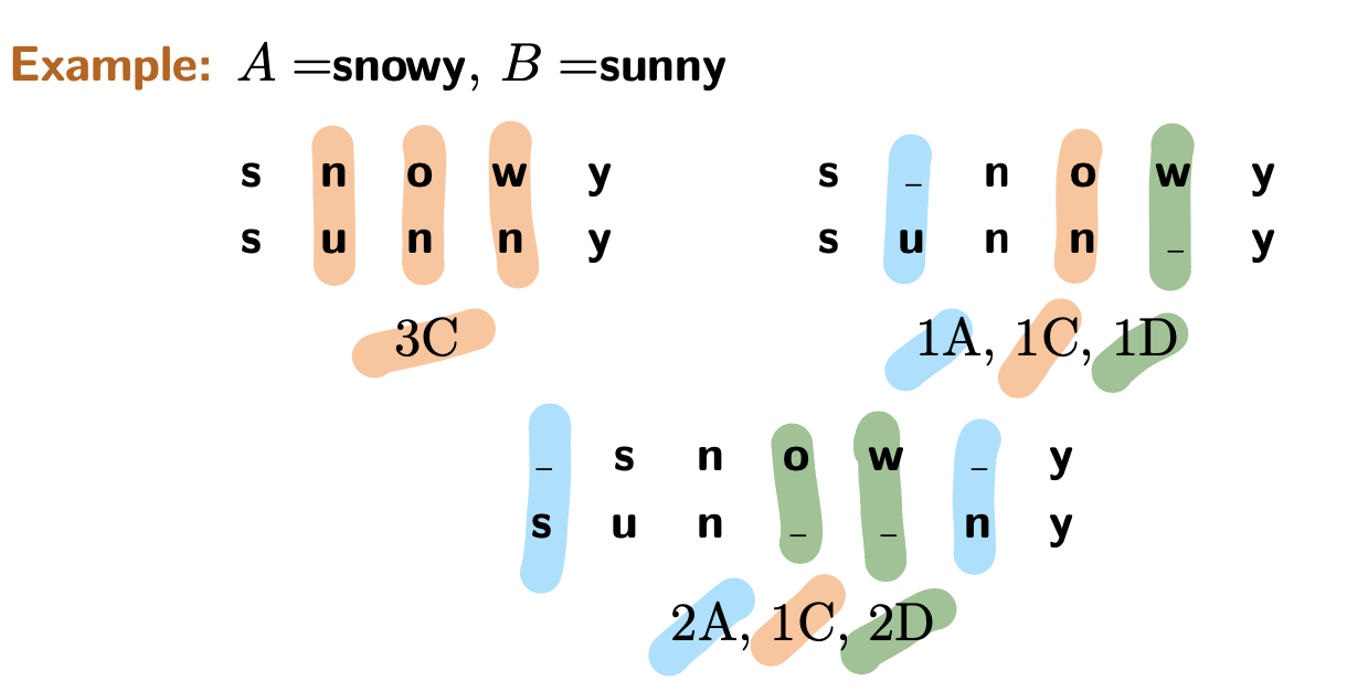
- from slide, first alignment need 3 changes so we have 3C
- then its 1A, 1C and 1D
- 1A being let’s say we missed typed a character, so we can add u
- 1C being we change o to n
- 1D being we typed an extra character w, so if we delete it, we will get sunny.
- last one … 2A, 1C, 2D
- 2A: we add s and n
- 1C: we change s to u (he forgot to put it in picture above)
- 2D: we delete o and w which one is the minimum?
You must list all the possible alignments and give the best!
Prof’s notes:
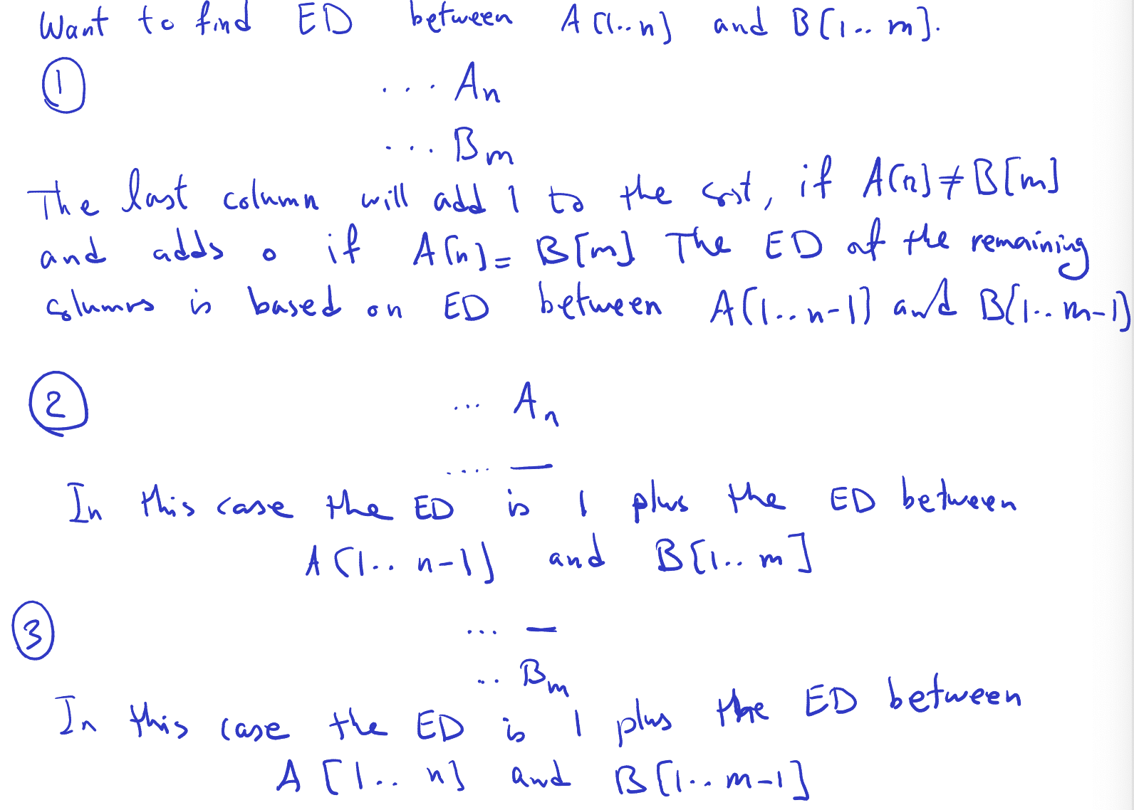
- We want to find ED between and . Three cases may happen:
-
- Align last character of A with last character of B. So is aligned with .
- The last column will add to the cost, if and adds if . The ED of the remaining columns is based on ED between and
-
- is not aligned with .
- In this case, the ED is 1 plus the ED between and
-
- is not aligned with at the end
- In this case, the ED is 1 plus the ED between and
This can be generalized to other indices. Let’s define an array at size and between and :
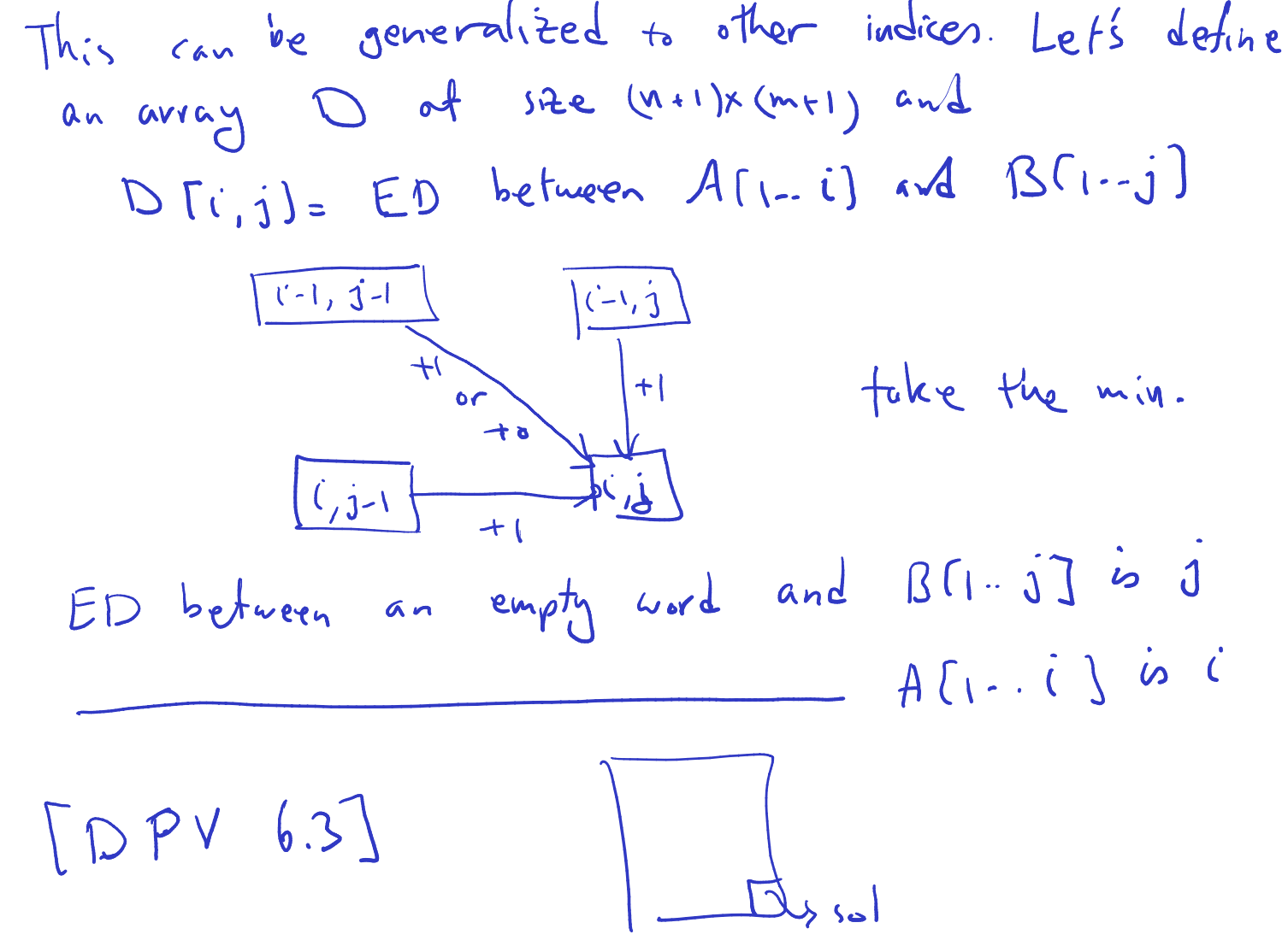
- What else does he need to tell us?
- Base case: ED between an empty word and is . ED between an empty word and is .
- Solution at bottom right cell.
Prof does have an example, but he doesn't have time to go through. Go to DPV 6.3 with an example of this for it to make more sense!
The recurrence:
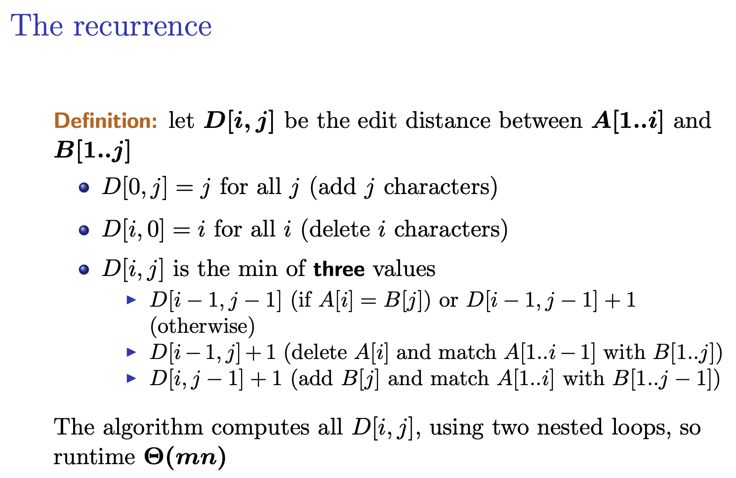
Definition
Let be the edit distance between and
- for all (add characters)
- for all (delete charracters)
- is the minimum of three values
- (if) or (otherwise)
- (delete and match with )
- (add and match with ) The algorithm computes all , using two nested loops, so runtime .
The recurrence relation provided defines the edit distance between two strings and in terms of smaller subproblems. Here’s a breakdown of the recurrence:
- Let be the edit distance between the prefixes and .
- Base cases:
- : The edit distance between an empty string and is because it requires adding characters to transform the empty string into .
- : The edit distance between and an empty string is because it requires deleting characters from to make it empty.
- Recurrence relation:
- is the minimum of three values:
- if : This corresponds to a substitution operation where is replaced by .
- : This corresponds to a deletion operation where is deleted, and we find the edit distance between and .
- : This corresponds to an insertion operation where is added to , and we find the edit distance between and .
- is the minimum of three values:
- The algorithm computes all values using two nested loops, iterating over all possible prefixes of the strings and , resulting in a runtime of , where and are the lengths of the strings and respectively.
Don't really understand why
D[i-1,j]+1is deletion operation whereA[i]is deleted andD[i,j-1]+1is insertion ofB[j]...???
Optimal Binary Search Trees
I Skipped over this Optimal Binary Search Trees when reviewing lectures!!!
Make sure to review for the finaltodo and take notes. Didn’t take notes either.
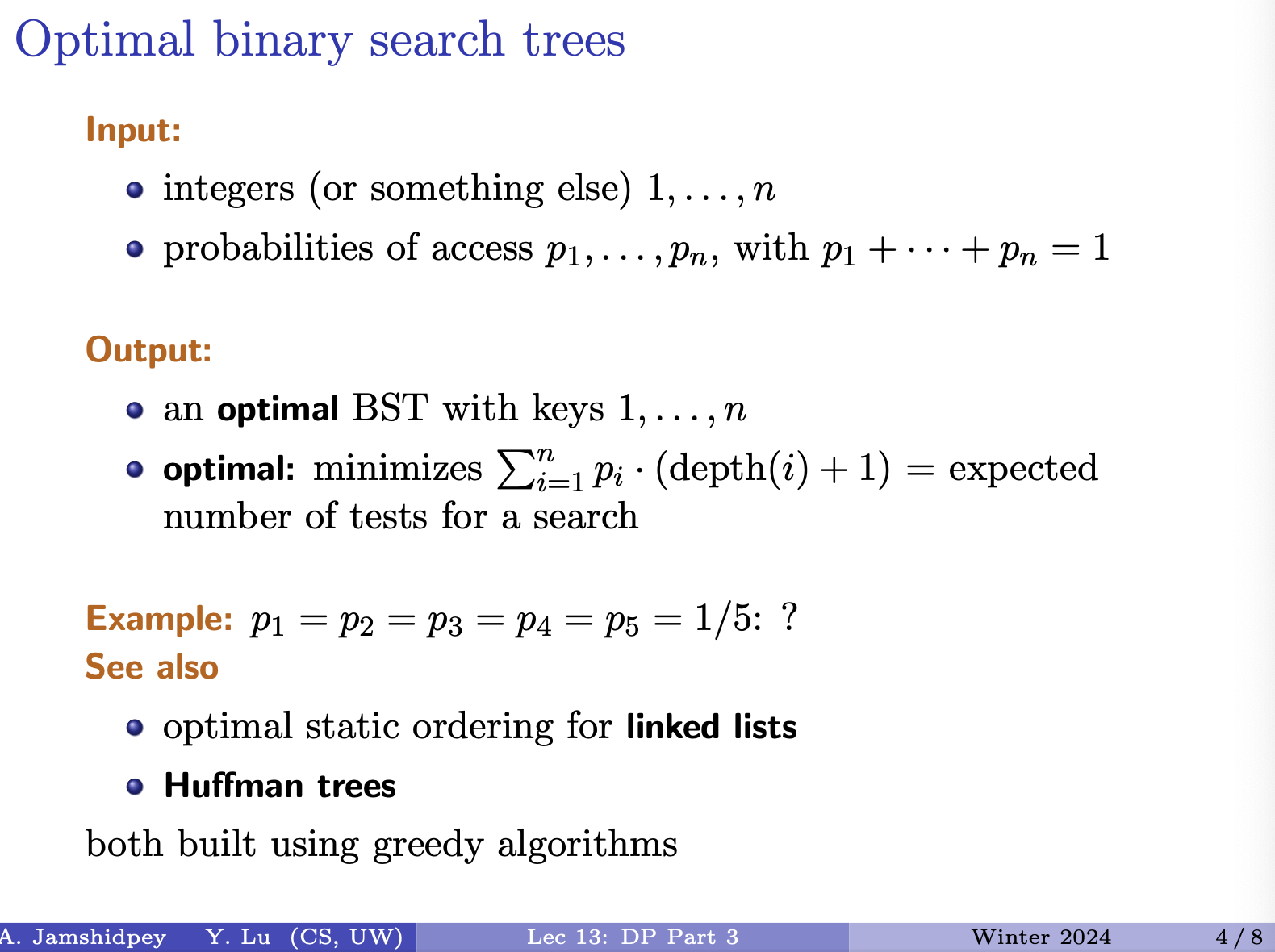
Keep the things you need close to yourself: MVT works on linked list. Seen in CS240.
There is something like this in the binary search trees.
- where can we access easily? The root
- must be multiplied by the probability
Example in this slide:
- Insert drawn picture
- For first tree: Compute:
- Didn’t have time to note the right side left one is better!
Does the greedy works here? No, since we are doing programming dynamic duh.
Prof’s notes:
- Greedy doesn’t work. Why?
- Insert picture (it’s the left tree)
- put the key with the highest probability in the root.
- So we put 5 in the root
- Then we pick 3 since it’s the largest in the rest
- Then 4
- After, that between 2 and 1 we choose 2.
- Lastly we put in 1.
So he has left and right tree.
- Left tree value is:
- Right tree: value is:
So greedy failed since it’s the left tree (in the picture).
Define to be the minimal cost for items to .
Take an item , between and and put it in the root. (my subproblems are from to )
Insert picture:
What are 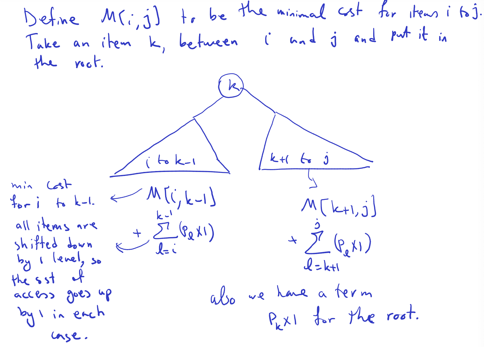
- if we look at the left, its a binary search tree, , every single node has one extra work, since we have pushed the whole tree down (look at the picture)
- main cost for to .
- all items re shifted downby 1 level so the s.t. of access goes up by 1 in eah case.
- Right side:
- to
- also we have a term for the root.
Stoped on 4/8 slide
Prof talked about the midterm.
- Question 2: easy divide-and-conquer, should just consider the intersection of the right and left side and that’s it
- Question 3: he shouted was gonna be in glass
- Question 4: True or false question
- Then he proceeded to show a graph of Assignment Average vs. Midterm Score. Not normal. 100 on assignment but 30 on the midterms… that’s a lot of people 200+ students
- They decided that if you do better on the final, they will use our final exam grade and discounting the midterm.
- He will fix the grades, don’t worry about the grades, worry about learning. What a chad.
Tues Mar 12, 2024
Prof redrew the graph: (reinsert the graph)
- The above formula is for any and we have to choose so that it gives the min value. So we try for all :
We also define … (to finish)
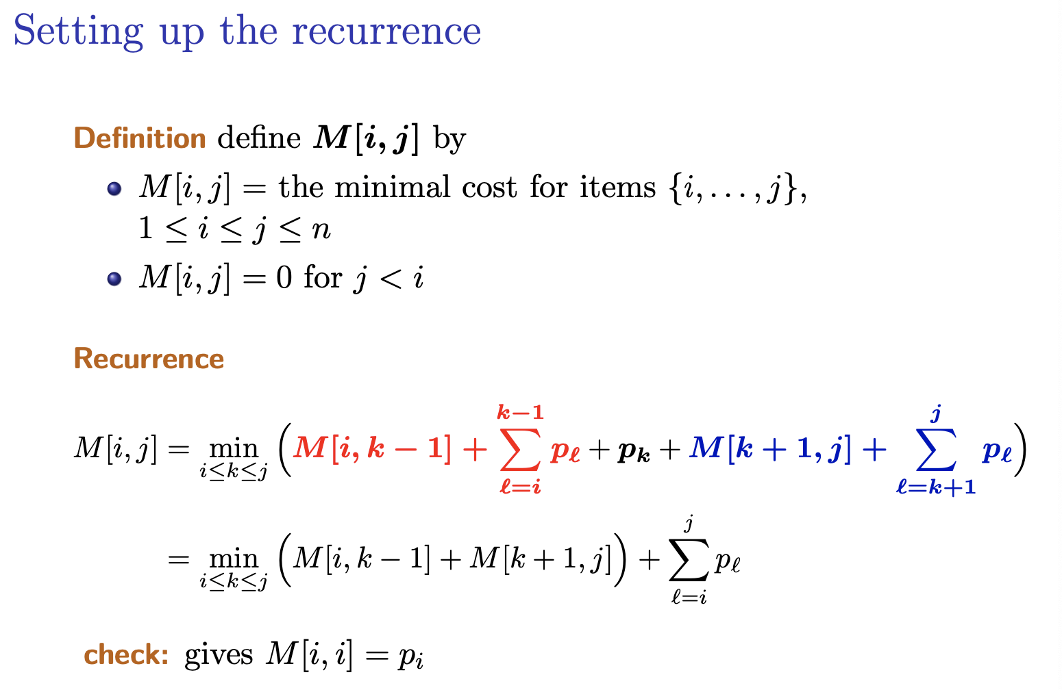
Algorithm: Pseudocode
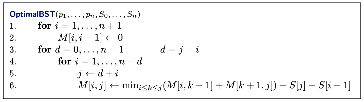
- : is a comment, we don’t overwrite the value of
He is not trying to solve the problem. Focusing on finding recurrence relation for DP.
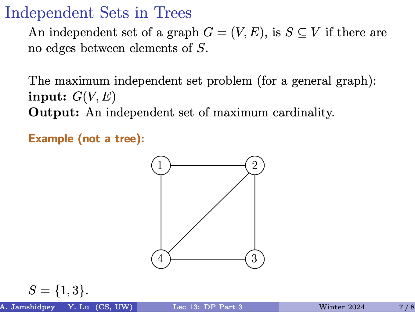
- S is a subset of V
- Independent: any two vertex I pick in S, they are not connected immediately by an edge. SHouldn’t be directly connected. Yes you can find a path.
- Cardinality is unique. Set is not necessarily unique. Size is indeed unique. The largest.
- 2 can’t go inside S? 4 has the same property, then you can add 1, 2 or 3.
- So the size is 2, and
- If I give you a tree, solve the problem? Think about an approach.
- DP has subproblems and trees have subtrees
- What he thinks of it: Step back and look at the objects from afar. Focus on one object and transfer the problem into subproblems.
- We choose the root. If it’s not in the tree, where can i find it? In subtrees. If the root is in the solution, where do we get the solution (should come from somewhere in the tree) so children are definitely not in the solution.
Prof’s notes:
- Given a tree (insert graph)
- Either the root appears in the a max ind. set or not
-
- : none of the children of can be in so, the remaining part of should come from subtrees rooted at grad children of . (insert picture on the left)
-
- In this case all elements of are from subtrees rooted at children of .
-
Write a formula for this recurrence relation:
- How do you refer to a subtree? (insert example tree). Just refer to the root. Say: the subtree rooted at a. The node is unique.
- Definition: is the size of the max independent set of the subtree rooted at .
- First sum: If is in max ind. set
- Second sum: If is not in max ind. set.
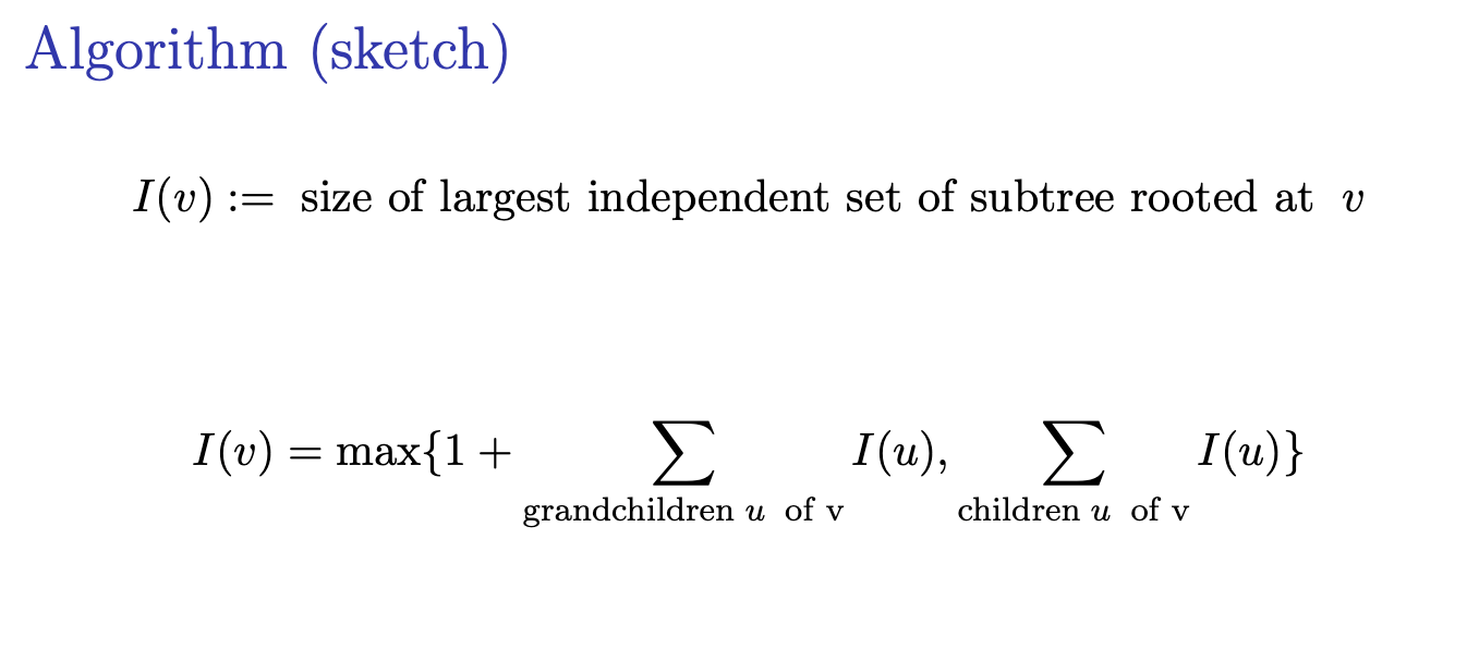
- Basically this slide^
Lecture 14 - Dynamic Programming - Part 4
The Bellman-Ford Algorithm
- source is fixed
- if no negative cycle, computes all distances δ(s, v)
- can detect negative cycles
- very simple pseudo-code, but slower than Dijkstra’s algorithm
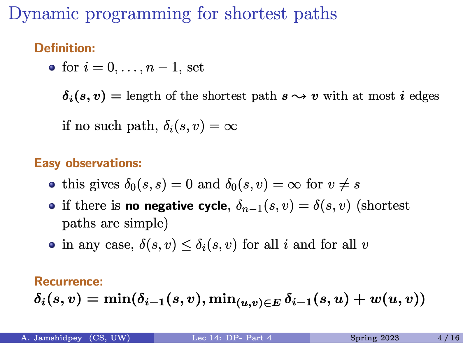
Definition:
- for , set
- n is number of vertices, and m is the number of edges
- length of the shortest path with at most edges if no such path
- I guess you initialize it to infinity at the beginning, so therefore, if you didn’t find a path? or shortest path? (what’s the difference) then you return for this the starting point to this vertex.
Easy observations:
- this gives and for
- If we want to use no edges, we have 0 which is the length of the path
- if there is no negative cycle, (shortest paths are simple)
- will be the value that you want, if no negative cycle
- why is it ?
- in any case, for all and for all
- easy observations
- represents the length of the shortest path from the source vertex to vertex in the graph. This is the optimal shortest path distance.
- represents the shortest path length from to that uses at most edges. This is the length of the shortest path with at most edges.
- one represents the optimal shortest path distance, and the other is the length
In this course, we don't allow self loops
Simple Path
In a simple path, no vertex can be repeated. Therefore, if there are vertices in the graph, the longest simple path from the source vertex to any other vertex will visit at most distinct vertices.
Recurrence:
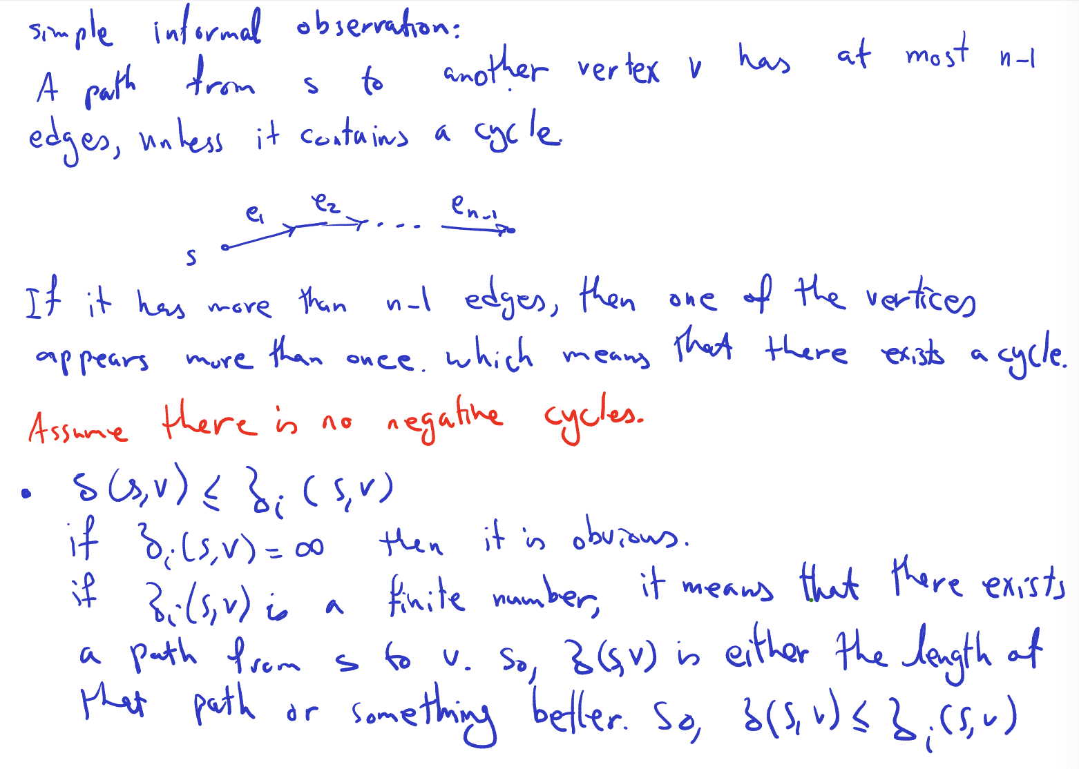
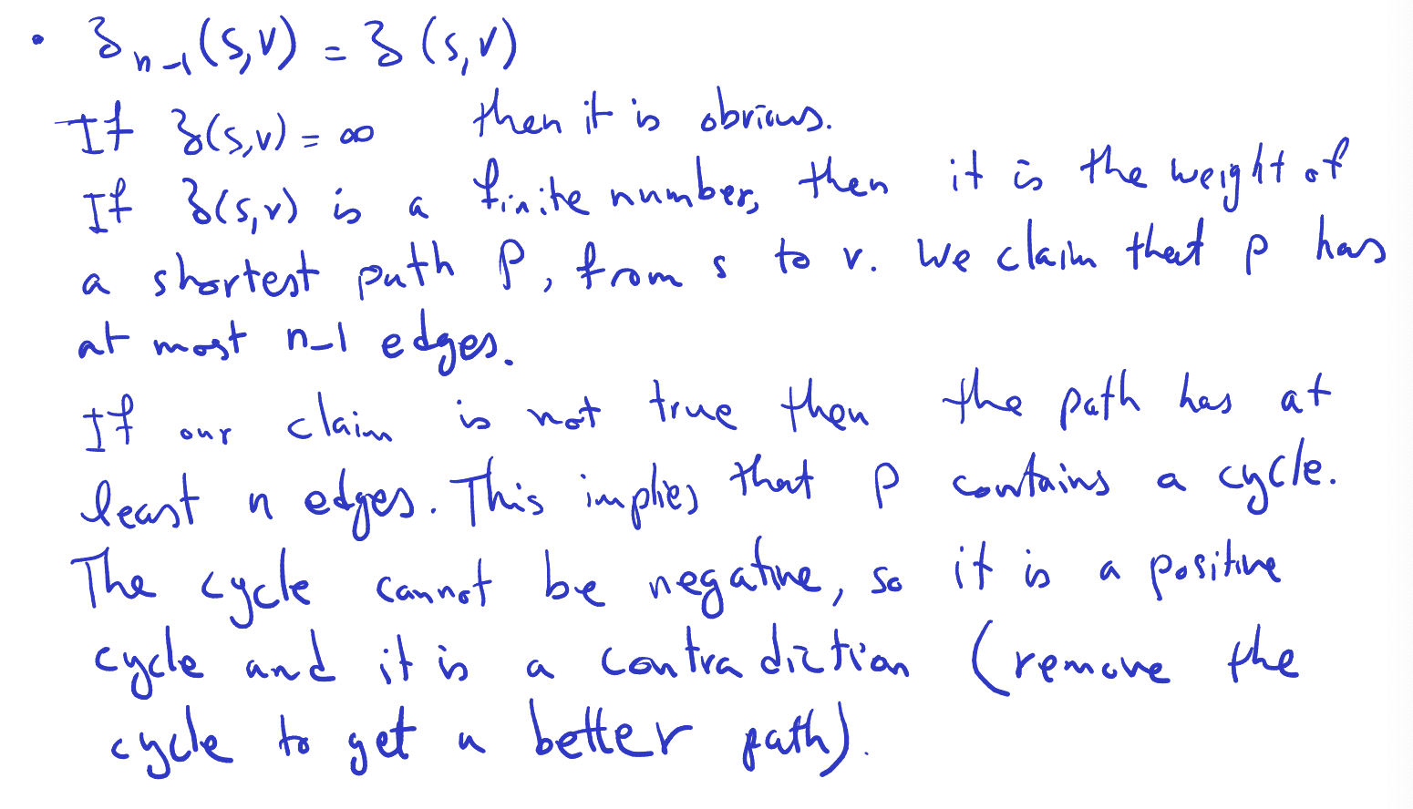
Now, why these observations hold?
- Simple informal observation:
- A path from to another vertex has at most edges unless it contains a cycle
- (insert picture of path he drew)
- if it has more than edges, then one of the vertices appears more than once which means that there exists a cycle
- (insert picture of path he drew)
- Assume there is no negative cycle!!
- First observation:
- If then it is obvious
- If is a finite number, it means that there exists a path from to . So, is either the length of that path or something better. So,
-
- If then it is obvious
- I have no paths
- If is a finite number, then it is the weight of the shortest path from to . We claim that this has at most edges.
- If our claim is not true, then the path has at least edges. This implies that contains a cycle. The cycle cannot be negative according to my assumption. So it is a positive cycle and it is a contradiction (remove the cycle to get a better path).
- We need the recurrence relation to find
- If then it is obvious
- A path from to another vertex has at most edges unless it contains a cycle
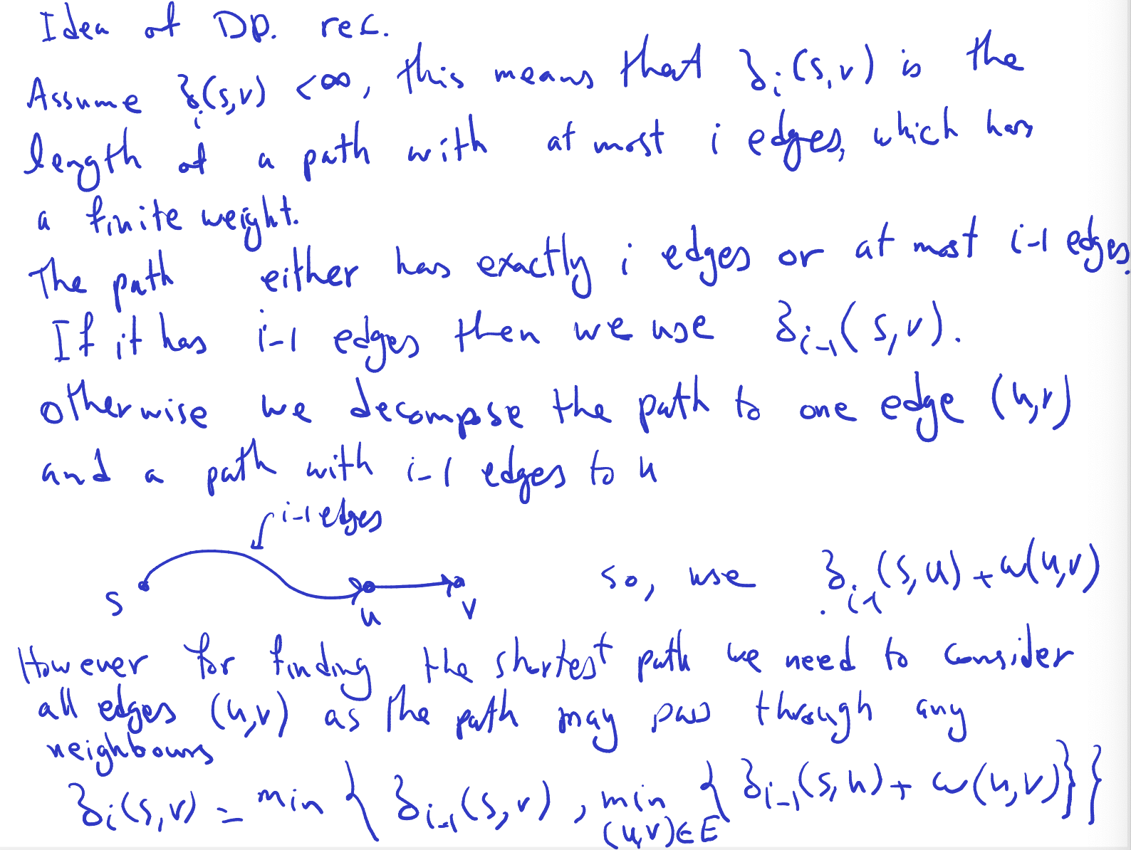
Idea of DP recurrence:
- Assume , this means that is the length at a path with at most edges which has a finite weight.
- The path either has exactly edges or at most edges.
- If it has edges then we use
- Otherwise, we decompose the path to one edge and a path with edges to
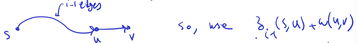
- So we use
- However, for finding the shortest paths we need to consider all edges as the path may pass through any neighbours.
where represents the set of edges in the graph, and represents the weight of the edge .
- Decomposition of Paths:
- If the shortest path from to contains exactly edges, then .
- If the shortest path from to contains at most edges, then we decompose it into two parts:
- The first part is an edge .
- The second part is a path from to using at most edges.
- Dynamic Programming Recurrence:
- To compute , we consider two cases:
- The shortest path from to using at most edges contains exactly edges. In this case, .
- The shortest path from to using at most edges contains an edge , where is a neighbour of . We try all possible neighbours of and compute the shortest path length from to using at most edges, then add the weight of edge .
- We take the minimum of these values to ensure we find the shortest path distance.
- To compute , we consider two cases:
So basically the two cases considers if we found it or we need to add another edge (path) and we find the shortest one. And add it to the solution. Something like that.
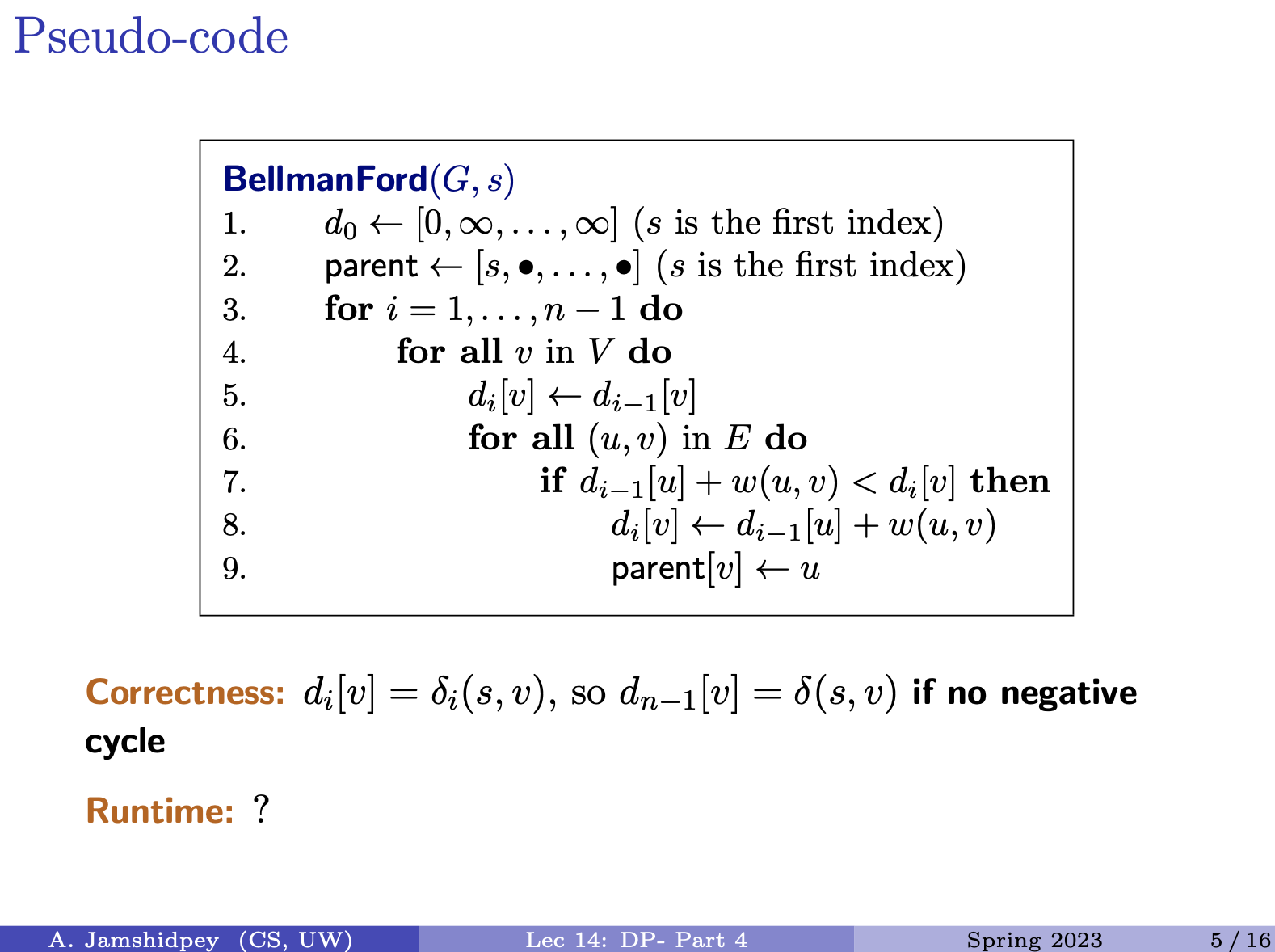
- for each we need to through each of the nodes (the vertices), then for all the neighbours of , we check
- go through every possible edges and we check (the if statement)
- There is too many arrays: and line 6: we go to all of u going into . Compute all the in neighbours.
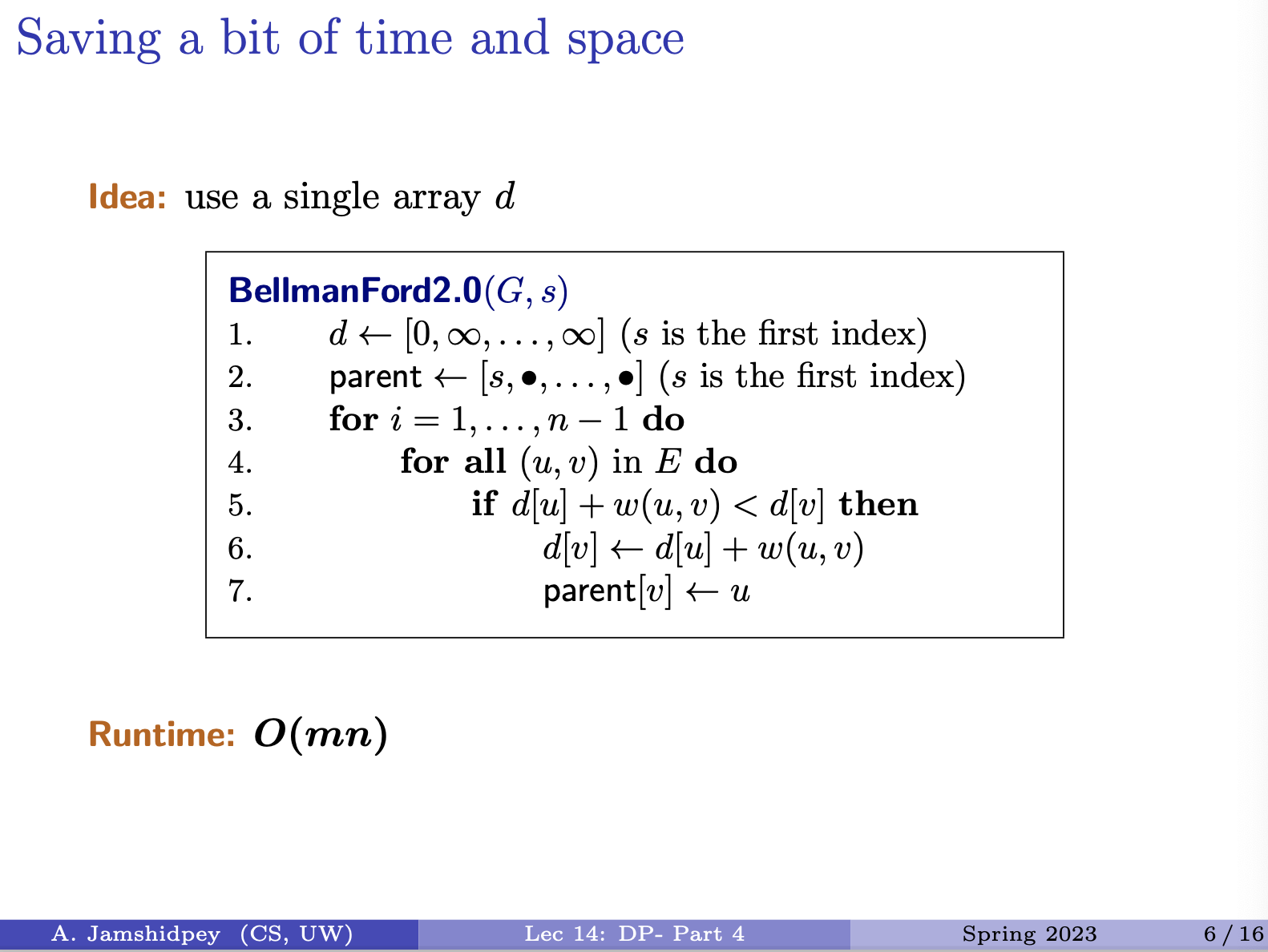
- d is array that we have, this time, we dont have d1, d2.
- Don’t care in what order we do it, in line 4, we are just looking at all edges. Pick the edges in any order you want
- Lines 5-7: is there a shorter paths: Seen in Dijkstra’s algorithm, which is the relaxation step.
Example: (Do it yourself)
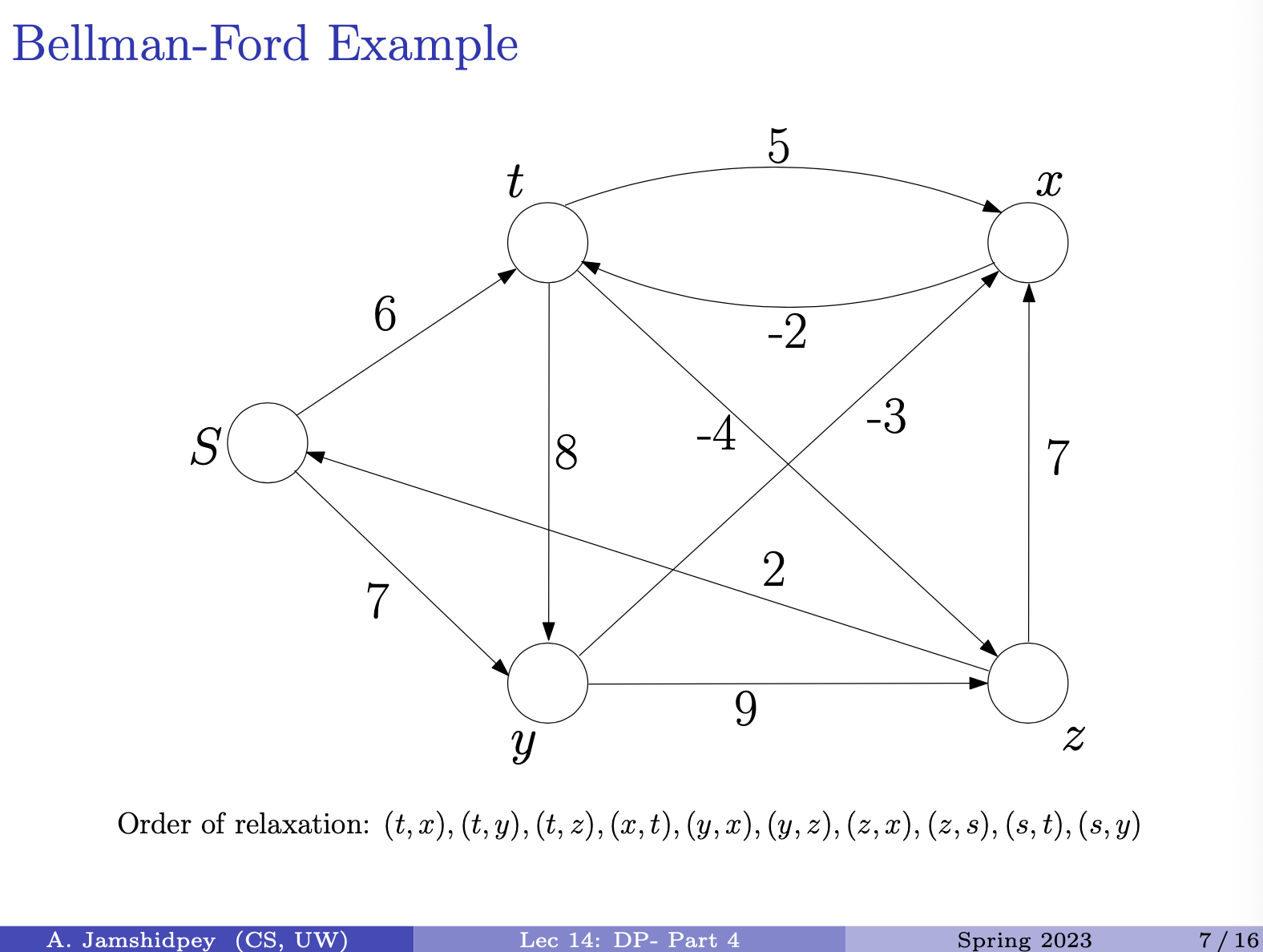
- change this slide, i think the prof updated it
Thu March 14 2024
Saving a bit of time and space
Idea: use a single array
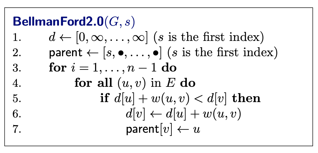
Runtime:
Insert prof’s notes:
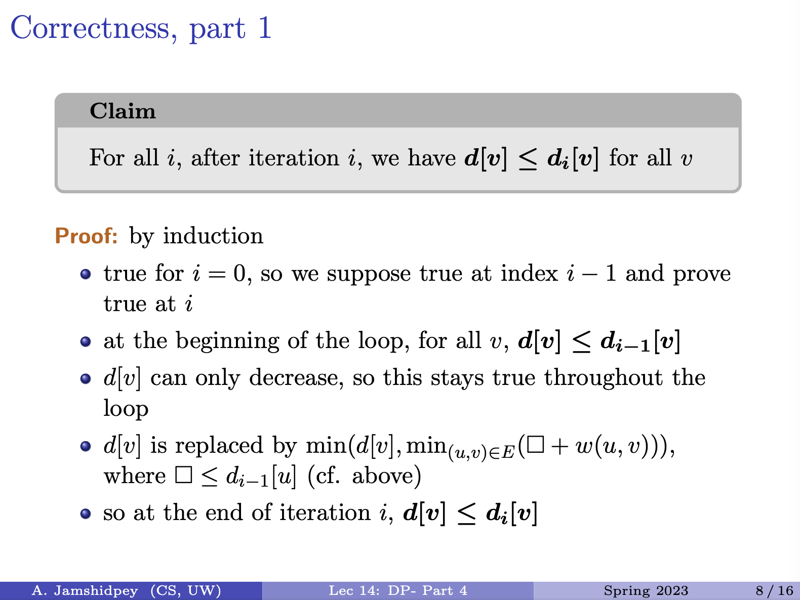
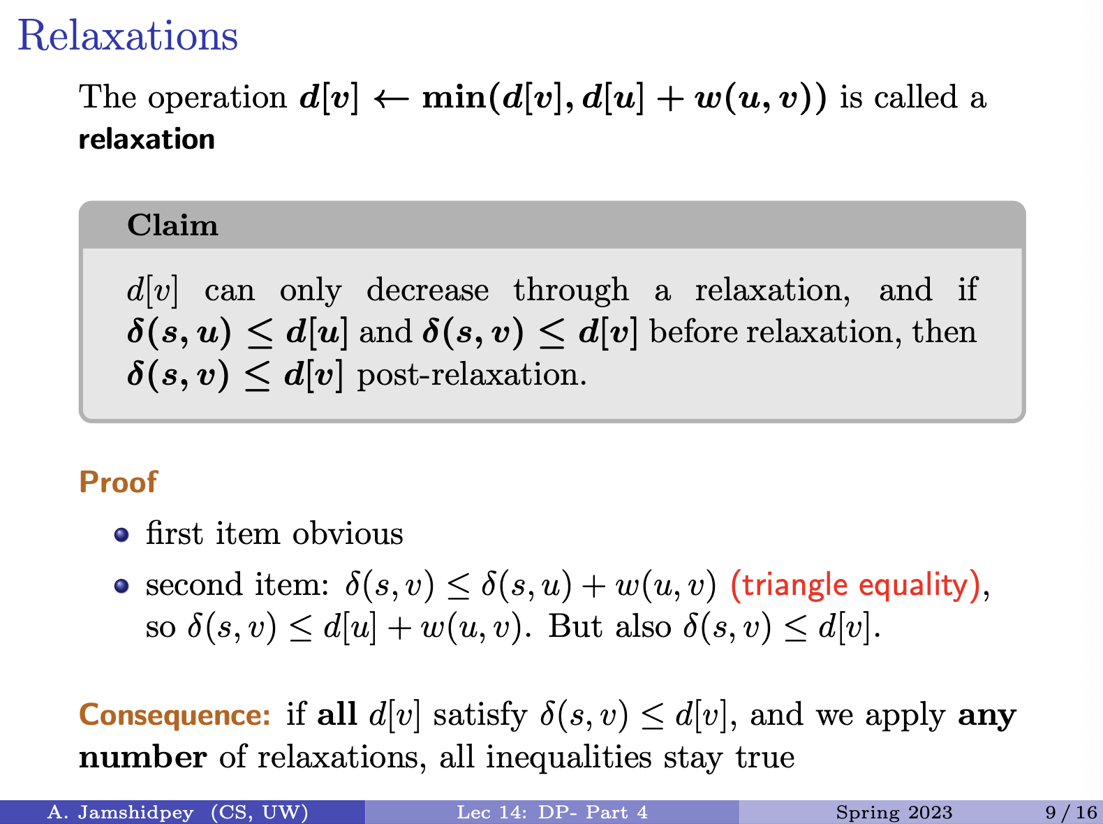
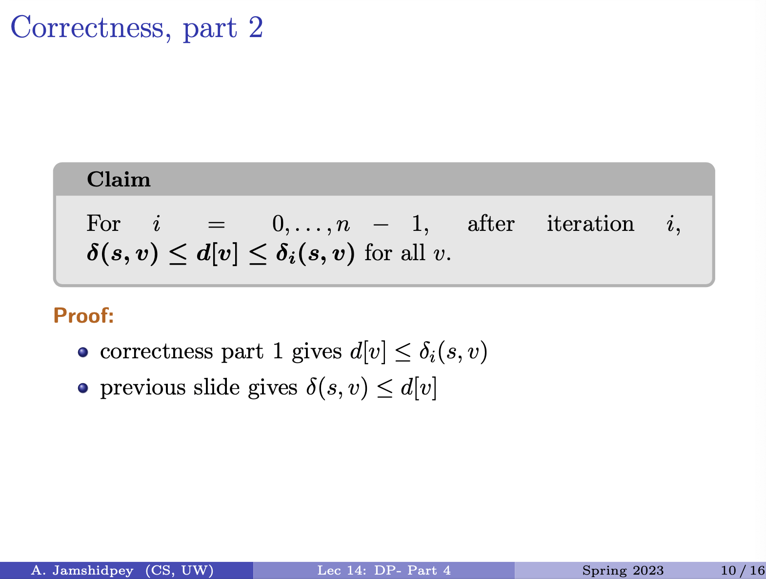
Summary
The Floyd-Warshall algorithm
- no fixed source: computes all distances
- negative weight OK but no negative cycle
- very simple pseudo-code, but slower than other algorithms
- another application of dynamic programming
Remark: doing Bellman-Ford from all takes ).
Looking at subsets of vertices
- Bellman-Ford uses paths with fixed numbers of steps.
- Floyd-Warshall restricts with vertices can be used
Insert prof’s notes: Floyd-Warshall recurrence relation
Dude drew a matrix in class. Insert that. Then compute .
- Examples are from CLRS.
Tue March 19 2024
Lecture 15: Polynomial Time Reduction
Only focus on decision problem in this module.
Decision Problem: Given a problem instance , answer a certain question “yes” or “no”.
Problem Instance: Input for the specified problem.
Problem Solution: Correct answer (“yes” or “no”) for the specified problem instance. is a yes-instance if the correct answer for the instance is “yes”. is a no-instance if the correct answer for the instance is “no”.
Size of a problem instance: is the number of bits required to specify (or encode) the instance .
Polynomial Reduction
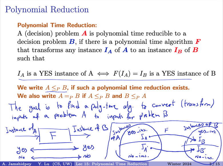
is a YES instance of is a YES instance of B.
We write , if such a polynomial time reduction exists. We also write if and
Polynomial Time Reduction
A decision problem is said to be polynomial time reducible to another decision problem , denoted as , if there exists a polynomial time algorithm that can transform any instance of into an instance of such that:
- If is a “yes-instance” of , then is a “yes-instance” of .
- If is a “no-instance” of , then is a “no-instance” of BB.
In essence, a polynomial time reduction allows us to solve problem by transforming its instances into instances of problem , solving problem , and mapping the solution back to the original problem.
Prof’s notes:
- The goal is to find a poly-time algorithm to convert (transform) input of a problem to inputs for problem .
Padlet Activity: Assume and are decision problems and we are given:
- an algorithm , which solves in polynomial time,
- a polynomial reduction , which gives Design a polynomial time algorithm to solve .
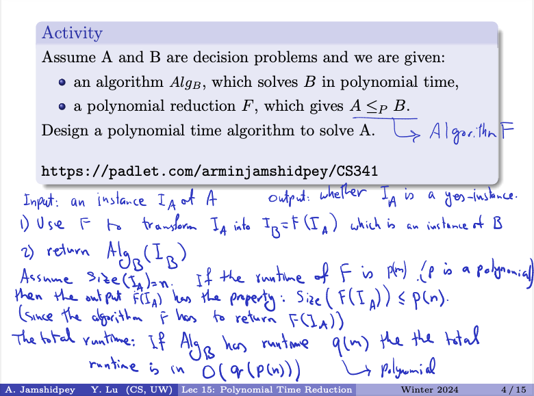
Input an instance of . Output whether is a yes-instance
- Use to transform into which is an instance of .
- return
The cost of returning is already considered. So if the cost is then .
Polynomial time refers always to the input. So here, it is in respect to ?
Assume . If the runtime of is (p is polynomial) then the output has the property: . (since the algorithm ) has to return .
The total runtime: If has runtime (polynomial) the total runtime is in
- Here is polynomial in terms of input of but we want to relate it to the input of apparently.
Analysis
- Size of Input Instances: When we discuss polynomial time complexity, it’s indeed in terms of the size of the input. If , it means has bits.
- Transformation by F: The polynomial-time reduction algorithm transforms into . Since runs in polynomial time, , where is a polynomial function.
- Runtime of : The algorithm can solve problem in polynomial time. Let’s say its runtime is , where is the size of the input for .
- Total Runtime: When we apply to , the size of the input is , which is bounded by a polynomial in terms of . Thus the total runtime is . Approach is correct, that is to solve problem using the polynomial-time reduction and the algorithm for problem . The total runtime is indeed , where is a polynomial runtime of , and is a polynomial bounding size of the transformed instance .
Transitivity Of Polynomial Time Reductions
Lemma
and
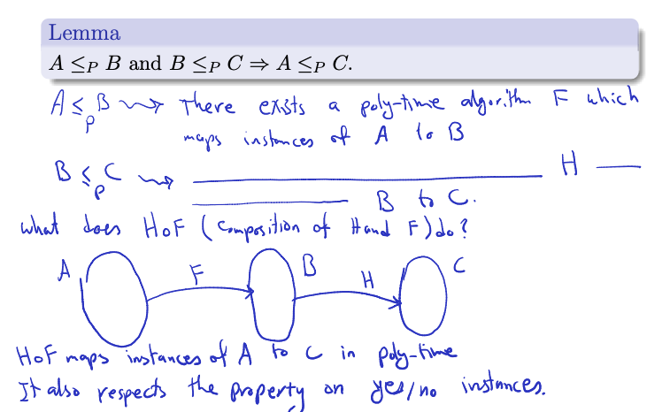
Proof:
- There exists a poly- time algorithm which maps instances of to .
- There exists a poly-time algorithm which maps instances of to .
- What does (Composition of and ) do?
Insert picture
- maps instances of to in poly-time. It also respects the property on yes/no instances.
Sanity Check
The composition of and , denotes as , essentially applies the transformation first, followed by the transformation . In other words, it maps instances of problem to instances of problem .
Proving Hardness Using Polynomial Reduction
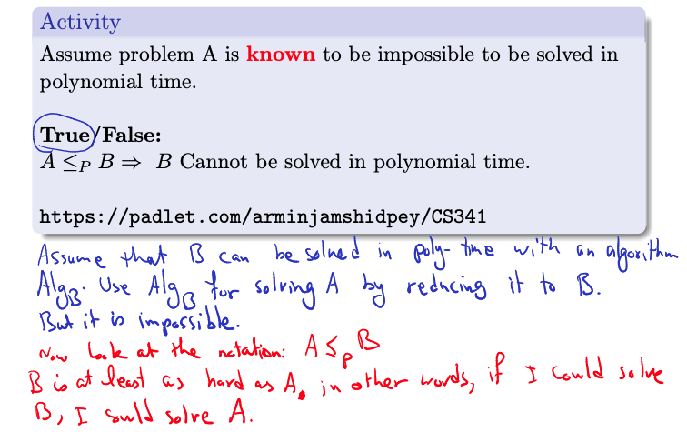
Activity: Assume problem is known to be impossible to be solved in polynomial time. True/False: Cannot be solved in polynomial time.
The answer is True. Assume that can be solved in poly-time with an algorithm. . Use for solving by reducing it to . But it is impossible.
Now look at the notation. . B is at least as hard as A, in other words, if I could solve , I could solve . B is harder to solve.
Summary:
In computational complexity theory, when we say that problem is polynomial-time reducible to problem (denoted as ), it means that we can efficiently transform instances of problem into instances of problem in polynomial time. In essence, this reduction implies that if we could solve problem efficiently (in polynomial time), then we could also solve problem efficiently by first transforming its instances into instances of BB and then using the polynomial-time algorithm for to solve them.
ahhhh
Assumption: Let’s assume that problem is known to be impossible to be solved in polynomial time. This implies that there is no polynomial-time algorithm capable of solving .
Implication: Now, if we have a polynomial-time reduction from to (i.e., ), and we assume that can be solved in polynomial time, it would imply that we could solve in polynomial time as well. This is because we could transform instances of into instances of using the polynomial-time reduction and then solve them using the assumed polynomial-time algorithm for .
Contradiction: However, this contradicts our initial assumption that problem cannot be solved in polynomial time. If cannot be solved in polynomial time, and we have a polynomial-time reduction from to , then also cannot be solved in polynomial time. This is because if were solvable in polynomial time, we would be able to solve in polynomial time, which contradicts our assumption about the hardness of .
Therefore, if problem is polynomial-time reducible to problem and problem is known to be unsolvable in polynomial time, it follows that problem cannot be solved in polynomial time either. This demonstrates how we can use polynomial reductions to infer the hardness of problems and establish relationships between their complexities.
Simple Reductions
The following three problems are equivalent in terms of polynomial-time solvability.
Maximum Clique
is a clique if, for all .
Input: and integer
Output: (the answer to the question) is there a clique in with at last vertices?
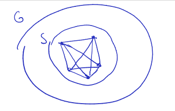
We’ve seen this Independent sets…
Maximum Independent Set (IS)
is an independent set if, for all .
Input: and an integer
Output: (the answer to the question) is there an independent set in with at least vertices?
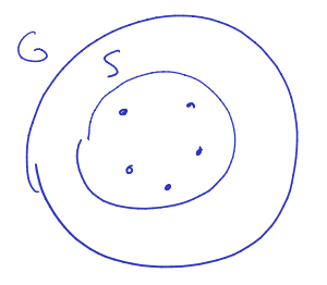
Minimum Vertex Cover (VC)
is a vertex cover if, for all .
Input: and an integer
Output: (the answer to the question) is there a vertex cover in with at most vertices?
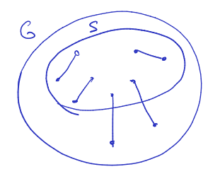
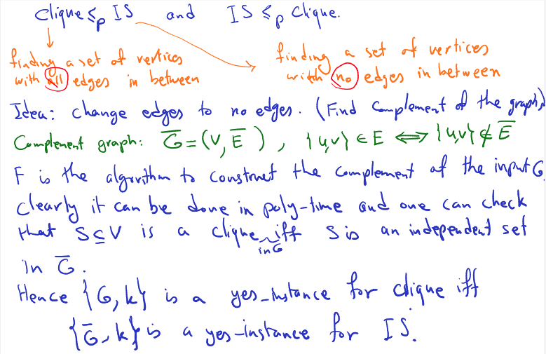
and
- Finding a set of vertices with all edges in between
- Finding a set of vertices with no edges in between
Idea: change edges to no edges. (Find complement of the graph).
Complement graph: , if and only if
is the algorithm to construct the complement of all the input . Clearly it can be done in poly-time and one can check that is a clique in is an independent set in .
Hence is a yes-instance for clique is a yes-instance for IS.
Summary key points
- Clique (Maximum Clique): Involves finding a subset of vertices where every pair of vertices is connected by an edge.
- Independent Set (Maximum Independent Set): Involves finding a subset of vertices where no pair of vertices is connected by an edge.
- Vertex Cover (Minimum Vertex Cover): Involves finding a subset of vertices such that every edge has at least one endpoint in the subset.
- basically, minimum set of vertices, so it covers all the edges in the graph.
- : By constructing the complement , where edges become non-edges and vice versa, we can transform instances of Clique into instances of IS. This reduction preserves the existence of cliques and independent sets.
- : Similarly, we can perform the same transformation to show that instances of IS can be transformed into instances of Clique, thus establishing the equivalence.
Conclusion: We can establish polynomial-time reductions between Clique, Independent Set, and Vertex Cover problems by utilizing the complement graph transformation.
Lemma
Assume is a graph.
is a vertex cover is an independent set in .
Too tired to write what he’s writing. Include picture of his proof I guess.
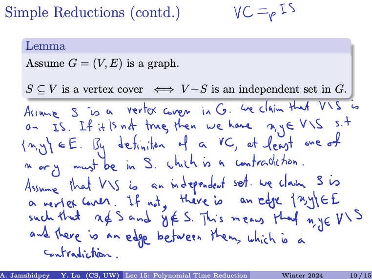
Prof’s proof of the lemma:
- Assume is a vertex cover in . We claim that is an IS. If it is not true, then we have such that . By definition of a CV, at least one of or must be in . Which is a contradiction.
- Assume that is an independent set. We claim is a vertex cover. If not, there is an edge such that and . This means that and there is an edge between them, which is a contradiction.
Ok so let me wrap my head around this. Proof:
- : is a Vertex Cover is and Independent Set
- We claim that is an independent set in .
- If is not an independent set, then there exists vertices such that .
- However, by the definition of a vertex cover, at least one of or must be in , otherwise, the edge would not be covered by .
- This contradiction implies that must be an independent set.
- : is an Independent Set is a Vertex Cover
- Assume is an independent set in .
- We claim that is a vertex cover of .
- If is not a vertex cover, then there exists and edge such that and .
- However, this contradicts the assumption that is an independent set, as and would both be in and adjacent, violating the independence property.
- This contradiction implies that must be a vertex cover.
Thu Mar 21 2024
Continues on slide 11/15. He was writing something…?
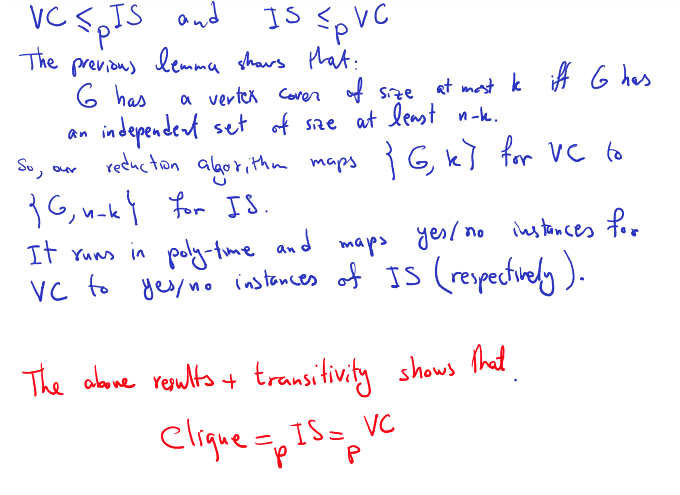
and
- The previous lemma shows that:
- has a vertex cover of size at most has an independent set of size at least .
- So, our reduction algorithm maps for VC to for IS.
- It runs in poly-time and maps yes/no instances for VC to yes/no instances of IS (respectively).
- The above results + transitivity shows that
Summarize main points
Equivalence between vertex cover (VC) and independent set (IS)
- The lemma establishes a clear equivalence between the existence of a vertex cover of size at most and the existence of an independent set of size at least in a graph .
- This equivalence allows us to construct a polynomial-time reduction from Vertex Cover to Independent Set and vice versa by transforming instances of one problem into instances of the other while preserving the yes/no answers.
- By applying the transitive property of polynomial reductions, we can conclude that the complexity of Vertex Cover, Independent Set, and Clique problems are equivalent, denoted as:
Implications:
- This equivalence implies that if any of these problems can be solved efficiently (in polynomial time), then all of them can be solved efficiently. Similarly, if any of them is proven to be NP-hard, then all of them are NP-hard.
More Simple Reductions
Hamiltonian Cycle (HC)
A cycle is Hamiltonian Cycle if it touches every vertex exactly once. Input: Undirected graph Output: (the answer to the question) Does have a Hamiltonian Cycle?
Hamiltonian Path (HP)
A path is a Hamiltonian Path if it touches every vertex exactly once. Input: Undirected graph Output: (the answer to the question) Does have a Hamilton path?
Proposition
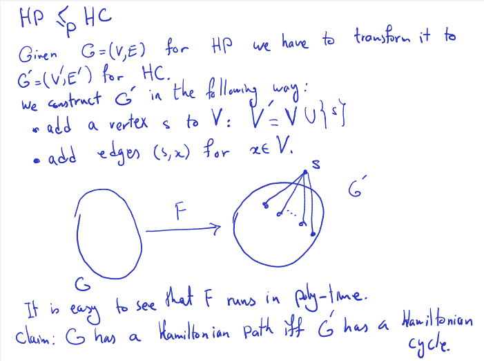
Proof:
- Note that he is not trying to solve it. Merely trying to reduce it so by finding an input for the RHS, we can find the input for the LHS.
If he adds an edge, his life would be good. Goal is to convert. Not to solve the problem?
The programming question is going to be similar to what the prof is going to do here.
If you have a large network, use MST.
He creates a node that connects to every vertex in including u and w.
- Given for HP we have to transform it to for HC.
- We construct in the following way:
- add a vertex to :
- add edges for
- If you give me graph G, convert it using F, to G’, just one extra vertex which is connected to everybody (insert the graph)
- It is easy to see that runs in poly-time.
Reduction from HP to HC
Easy to understand.
To perform the reduction, the algorithm adds a new vertex to the graph , which is connected to every vertex in , including the endpoints of the desired path in . This new graph is then constructed such that has a Hamiltonian cycle if and only if has a Hamiltonian path.
Implications:
- The reduction algorithm constructs from in polynomial time.
- The transformation ensures that has a Hamiltonian path if and only if has a Hamiltonian cycle, establishing the equivalence between the HP and HC problems
Claim:
Ghas a hamiltonian path if and only ifG'has a hamiltonian cycle.
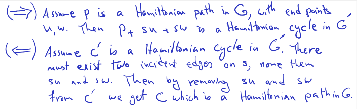
Proof:
- Assume is a Hamiltonian path in , with end points . Then is a Hamiltonian cycle in .
- Assume is a Hamiltonian cycle in . There must exist two incident edges on , name them and . Then by removing and from , we get which is a Hamiltonian path in .
Pretty straightforward.
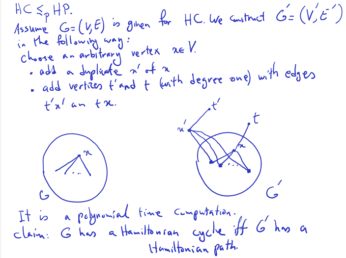
Now, let’s see .
Reduction is not about solving, but about reducing. Let’s say we have , and a path from u to w. Instead, he’s creating a hamiltonian path that starts and end on the two vertex he adds which is of degree one. If we want to add those two points what do we do.
So given a graph , you pick a random vertex , you want to create with the property being a copy of . So whoever was a neighbour of would be a copy of in . This can be done in polynomial time. Super easy. We also want to create those two nodes mentioned earlier. So we create vertex and with degree 1. This can be done in polynomial time. is connected to and is connected to . If we have a hamiltonian cycle in , then should be part of it, and some and . We can construct a hamiltonian path from to to , then to then got to then .
Prof’s notes:
- Assume is given for HC. We construct in the following way: Choose an arbitrary vertex
- add a duplicate of
- add vertices and (with degree one) with edges and .
- It is a polynomial time computation
Proof outline (sanity check)
- :
- Assume has a Hamiltonian cycle.
- Choose an arbitrary vertex from .
- Construct a graph by adding a duplicate vertex of and two new vertices and with degree 1.
- Connect to and to .
- Since has a Hamiltonian cycle, must be part of it.
- Hence, a Hamiltonian path in can be constructed starting from , traversing , and then visiting the edges of in the order of the Hamiltonian cycle, ending at .
- :
- Assume has a Hamiltonian path.
- If has a Hamiltonian path, it means that there exists a path that visits all vertices of exactly once.
- Since and are of degree 1 and adjacent to and respectively, this path must start at and end at .
- Therefore, the vertices visited in between and correspond to the vertices of .
- Hence, there exists a Hamiltonian cycle in .
Claim:
Ghas a Hamiltonian cycle if and only ifG'has a Hamiltonian path
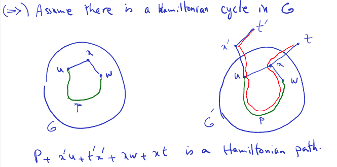
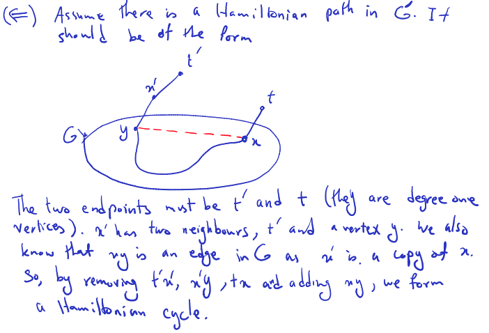
Proof:
- Assume there is a Hamiltonian cycle in and we want . So we still have Hamiltonian cycle.
- Of course, there are other vertices in the graph that he doesn’t need to draw because we care about the cycle.
- Then in , we see that in red, we have a Hamiltonian path. is a Hamiltonian path
- Assume there is a Hamiltonian path in . It should be of the form (insert picture). Basically . There must be an edge from x to y, because we have an edge from to y.
- The two endpoints must be and (they are degree one vertices). has two neighbours, and a vertex . We also know that is an edge in as is a copy of . So, by removing and adding , we form a Hamiltonian cycle.
If we don’t have and , something like this may happen (drawn in the box, but he fucking erased it, said something like he was gonna do a counterexample). We have a hamiltonian path here (in the cycle which is the transformed graph), but we can’t create a hamiltonian cycle. So we need and to start and end outside (where we want???).to-understand fully. It makes sense, but I’m trying to see if
An Important Problem
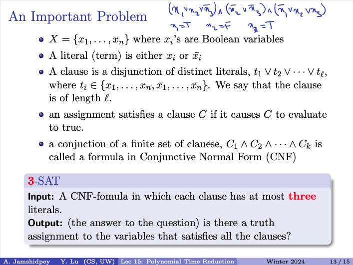
- where ‘s are Boolean variables
- A literal (term) is either or
- A clause is a disjunction of distinct literals, where . We say that the clause is of length .
- an assignment satisfies a clause if it causes to evaluate to true.
- a conjunction of a finite set of clauses, is called a formula in Conjunctive Normal Form (CNF).
3-SAT (Theorem Cook-Levin)
Input: A CNF-formula in which each clause has at most three literals.
Output: (the answer to the question) is there a truth assignment to the variables that satisfies all the clauses?
- the distinct literals, or ,… are all in
He gives an example, which gives a true value:
How doe we get each of these to be true. We can just grab one of the and checks if it is True?
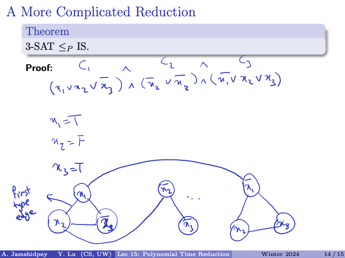
Theorem
3-SAT .
Let’s assign , then take to be True, therefore . In , we can only take and assign it to be true. Every time, he takes one out of the clause and make sure it doesn’t already have any connection with previous picks, no relations between these. Translate this in a graph, being picking a vertex such that each of the vertex we pick has are not connected to each other.
The thing he drew down there is called a first type edge. For each clause, create the number of nodes and connect each other. Then for second one, we connect them again. (If a clause only has one vertex, we don’t have to draw it or something.) For every single clause, we create a graph, not connected at first. We connect the clauses if they are negations of each other as seen below. (continue doing this).
Proof Outline
Reduction from 3-SAT to IS:
- Given a 3-SAT formula, construct a graph where each variable corresponds to a vertex in the graph.
- For each variable , create two vertices: and , representing the true and false assignments respectively.
- Connect the vertices corresponding to the literals in each clause. If a clause contains a literal , connect the vertices corresponding to and to the vertices corresponding to the other literals in the clause. This ensures that if one literal in the clause evaluates to true, the clause can still be satisfied.
- Ensure that vertices representing literals within the same clause are not connected directly. This prevents assigning conflicting truth values to literals within the same clause. The resulting graph represents a collection of disjoint sets of vertices, each set representing a clause in the 3-SAT formula.
- The objective is to find an independent set in this graph, where no two vertices in the set are adjacent. This corresponds to finding a truth assignment to the variables that satisfies all the clause in the 3-SAT formula.
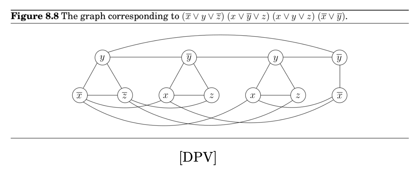
Tues March 26
He started with the last slide of Lecture 15. Include the picture and his annotations.
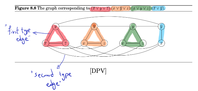
Make sure to connect the nodes between the literals if they are opposites of each other.
Transform the CNF into an independent set. There are two inputs, first input is the graph, then input integer k. And set k to the number of clause.
Take the true literals. If we choose to be true in the first clause. What’s the whole thing about the k set of independent set??
Prof’s notes:
- A CNF with clauses of length at must 3 is given. For each clause we form a triangle with vertices labeled as the literals of the clause.
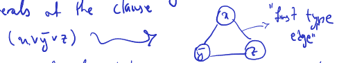
- A clause with 2 literals will be an edge from one to the other
- A clause with only one literal is easy to deal with.
- To force exactly one choice from each clause, we set to be the number of clauses.
- We have to make sure that we are not choosing opposite literals and in different clauses. So, we create an edge between any two vertices that corresponds to opposite literals.
- This contradiction takes polynomial time.
Summary
Graph Construction
- For Each Clause:
- For each clause in the CNF formula, create a triangle in the graph.
- Each vertex of the triangle represents a literal in the clause.
- Ensure that the literals within the same clause are not directly connected to each other to prevent conflicts.
- Handling Clauses with 2 Literals:
- For clauses with only two literals, create an edge between the two corresponding vertices in the graph.
- Handling Clauses with 1 Literal:
- Clauses with only one literal are easy to handle as they represent a single vertex in the graph.
- Connecting Opposite Literals:
- To ensure that opposite literals (e.g., and ) from different clauses are not chosen together, create and edge between any two vertices representing opposite literals.
Independent Set Construction
- Each set of vertices in the graph represents a clause in the CNF formula.
- The objective is to choose one vertex from each triangle (clause) such that no two chosen vertices are adjacent (i.e., represent literals in the same clause).
- Setting to be the number of clauses ensures that exactly one vertex is chosen from each clause.
Claim
Suppose the CNF formula has clauses. The formula is satisfiable if and only if there is an independent set of size in the graph.
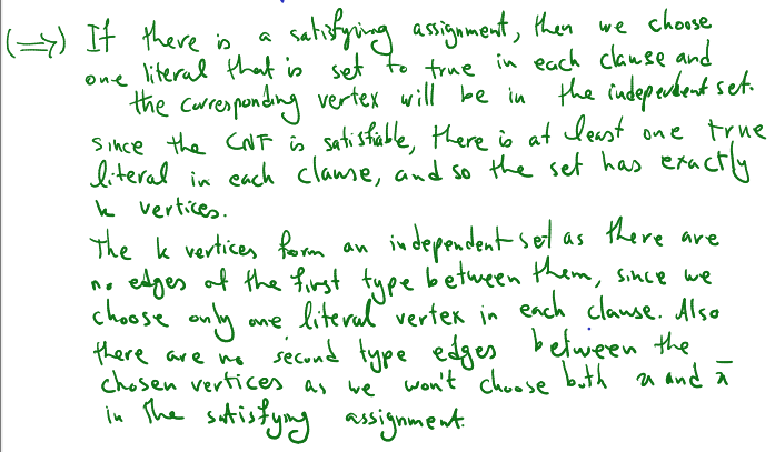
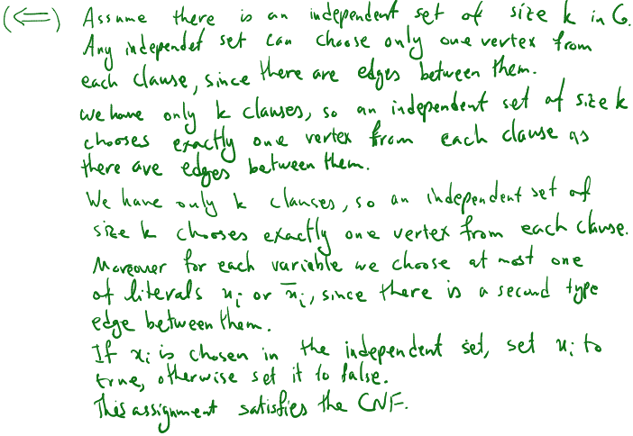
Proof:
-
- If there is a satisfying assignment, then we choose one literal that is set to true in each clause and the corresponding vertex will be in the independent set.
- Since the CNF is satisfiable, there is at least one true literal in each clause, and so the set has exactly vertices.
- The vertices form an independent set as there are no edges of the first type between them, since we choose only one literal vertex in each clause. Also there are no second type edges between the chosen vertices as we won’t choose both and in the satisfying assignment.
-
- Assume there is an independent set of the size in .
- Any independent set can choose only one vertex from each clause, since there are edges between them. We have only clauses, so an independent set of size chooses exactly one vertex from each clause as there are edges between them.
- We have only clauses, so an independent set of size chooses exactly one vertex from each clause.
- Moreover, for each variable we choose at most one of literals or , since there is a second type edge between them.
- If is chosen in the independent set, set to true, otherwise set it to false.
- This assignment satisfies the CNF.
Trying to understand explanation
Satisfiability of CNF formula:
- A CNF formula with clauses is satisfiable if there exists a truth assignment to the variables that satisfies all clauses simultaneously.
Independent Set in Graph:
- An independent set in the graph representation of the CNF formula corresponds to a selection of vertices (literals) from the graph such that no two selected vertices share an edge (representing conflicting literals within the same clause).
- The size of the independent set represents the number of clauses selected from the CNF formula.
Relationship:
- The claim asserts that the CNF formula is satisfiable if and only if there exists an independent set of size in the graph.
- If the CNF formula is satisfiable, then there exists a truth assignment satisfying all clauses, which translates to the existence of an independent set of size in the graph.
- Conversely, if there exists an independent set of size in the graph, then it corresponds to selecting one literal from each clause, ensuring that the selected literals satisfy all clauses simultaneously, thus proving the satisfiability of the CNF formula.
Lecture 16 - NP-completeness
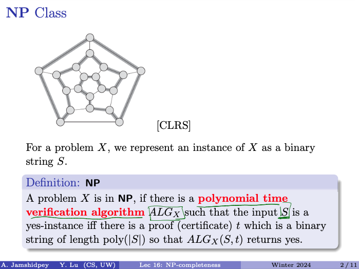
Counting the number of bits.
Definition: NP
A problem is in NP if there is a polynomial time verification algorithm such that the input is a yes-instance iff there is a proof (certificate) which is a binary string of length poly() so that returns yes.
Trying to Understand
Verification Algorithm:
- For a problem to be in NP, there must exist a verification algorithm that runs in polynomial time.
- This verification algorithm takes two inputs:
- The problem instance .
- A proof or certificate , represented as a binary string of length polynomial in the size of .
Polynomial Time Verification:
- The verification algorithm verifies whether the given instance is a “yes-instance” by checking the validity of the proof .
- If is indeed a “yes-instance” of the problem , there exists a proof such that returns “yes” in polynomial time.
Relationship with Yes-Instances:
- The problem instance is considered a “yes-instance” of if and only if there exists a valid proof such that returns “yes”.
- In other words, the existence of a valid proof serves as evidence that is indeed a “yes-instance” of .
The definition of NP highlights the significance of polynomial-time verification algorithms in determining whether a given problem instance belongs to the complexity class NP. Problems in NP are characterized by the existence of efficient verification procedures that can confirm the correctness of proposed solutions, given suitable proofs or certificates.
Examples
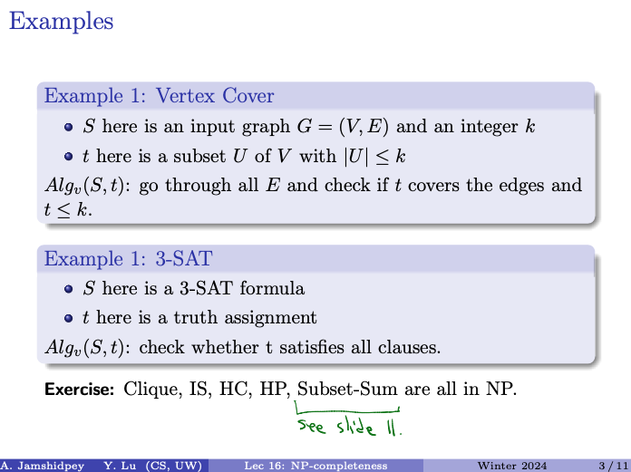
Example 1: Vertex Cover
- here is an input graph and an integer
- here is a subset of with : go through all and check if covers the edges and .
Example 2: 3-SAT
- here is a 3-SAT formula
- here is a truth assignment : check whether satisfies all clauses.
Exercise: Clique, IS, HC, HP, Subset-Sum are all in NP.
- is a solution to that problem (usually)
- So is some sort of instance of a 3-SAT formula or what????gap-in-knowledge
- Is 3-SAT NP?
- Yes, it is an NP problem
- Not all problems are in NP
See slide 11 for Subset-Sum:
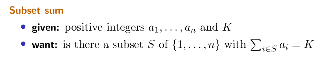
You can now refer to slide 11 without showing any proof? And allowed to use the information and do the assignment.
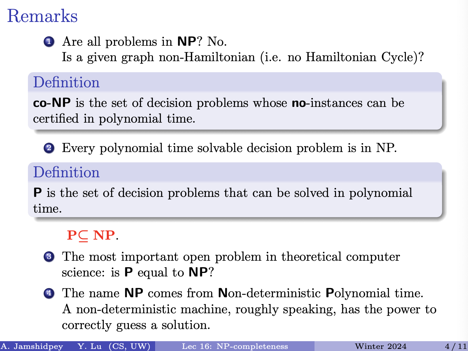
- We won’t see a lot of co-NP.
Definition
is the set of decision problems that can be solved in polynomial time.
- if you solve this problem, you can generate the certificate of that.
NP-completeness
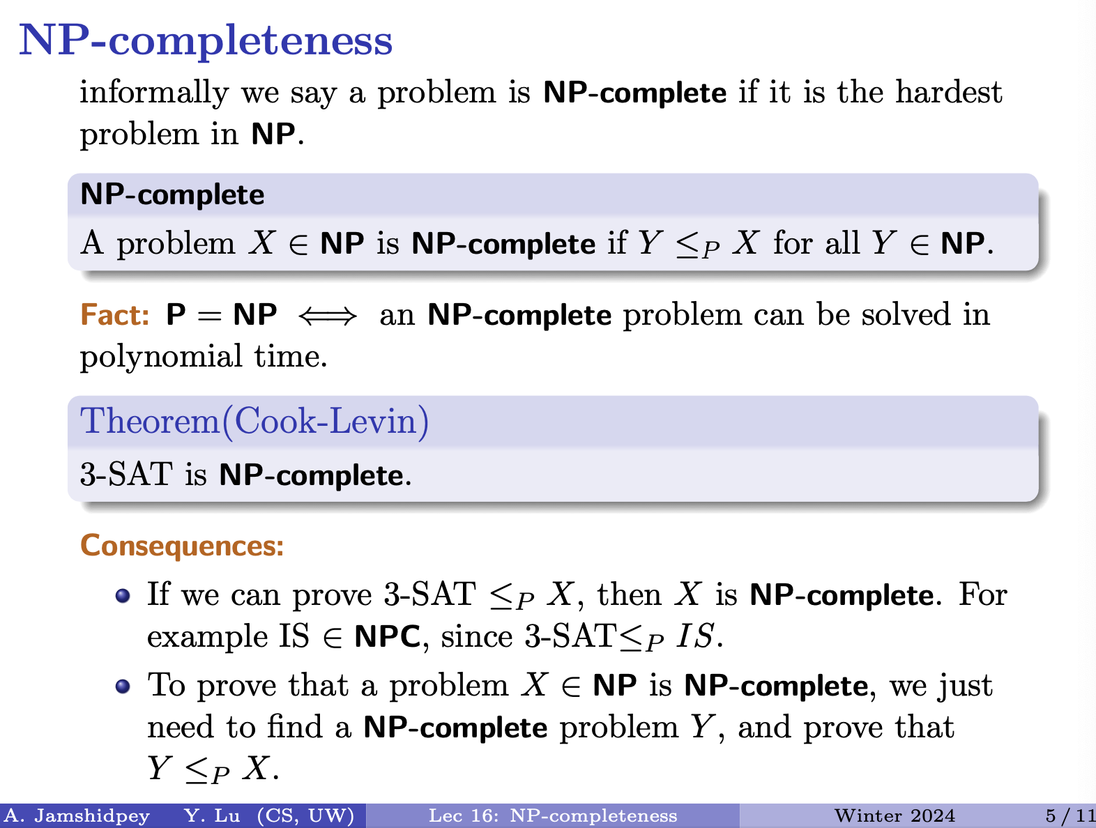
NP-complete
A problem is NP-complete if for all .
Fact: an NP-complete problem can be solved in polynomial time.
Theorem (Cook-Levin)
3-SAT is NP-complete.
Consequences:
- If we can prove 3-SAT , then is NP-complete. For example , since 3-SAT .
- To prove that a problem is NP-complete, we just need to find a NP-complete problem , and prove that .
Understanding...
Definition of NP-Completeness:
- A decision problem is said to be NP-complete if it belongs to the complexity class NP and every problem in NP can be reduced to in polynomial time.
- In other words, if there exists a polynomial-time reduction from any problem in NP to , then is NP-complete.
Implications of NP-completeness:
- NP-complete problems are among the hardest problems in NP, as they capture the computational complexity of all problems in NP
- If a polynomial-time algorithm can be found for any NP-complete problem, it would imply that , meaning every problem in NP can be solved in polynomial time.
Cook-Levin Theorem:
- The Cook-Levin theorem states that the 3-SAT problem is NP-complete.
- This theorem is significant as it provides a foundational example of an NP-complete problem and demonstrates that 3-SAT captures the computational complexity of all problems in NP.
Consequences: Identifying NP-Complete Problems
- To prove that a problem is NP-complete, one needs to demonstrate a polynomial-time reduction from a known NP-complete problem to .
Solving NP-Complete Problems:
- Solving an NP-complete problem efficiently would imply that , which is a major open question in computer science
- Therefore, many researchers focus on identifying efficient algorithms for specific NP-complete problems or approximating solutions to these problems.
- If we can solve B in polynomial time, we can solve A in polynomial time. Then if B is the hardest problem, every single NP problem can be reduced to B.
If we can solve an NP efficiently,
- Every NP problem can be reduced to max independent set.
- 3-SAT is proven to be reducible to IS
On exam:
- Show that your problem is NP
- If there exist an NP complete problem that can be reduced to yours.
- Then it is NP complete
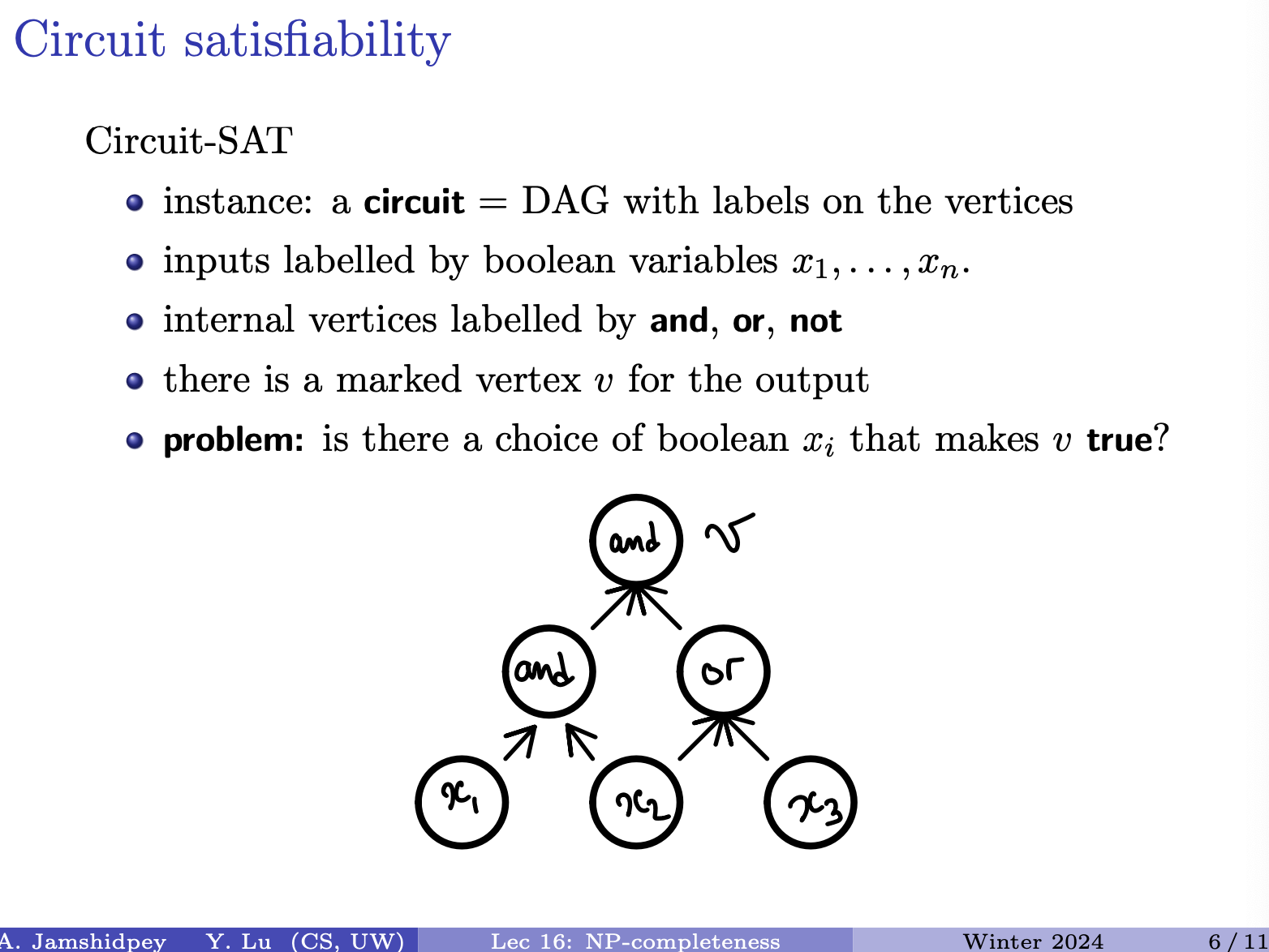
He created a red box? around true?
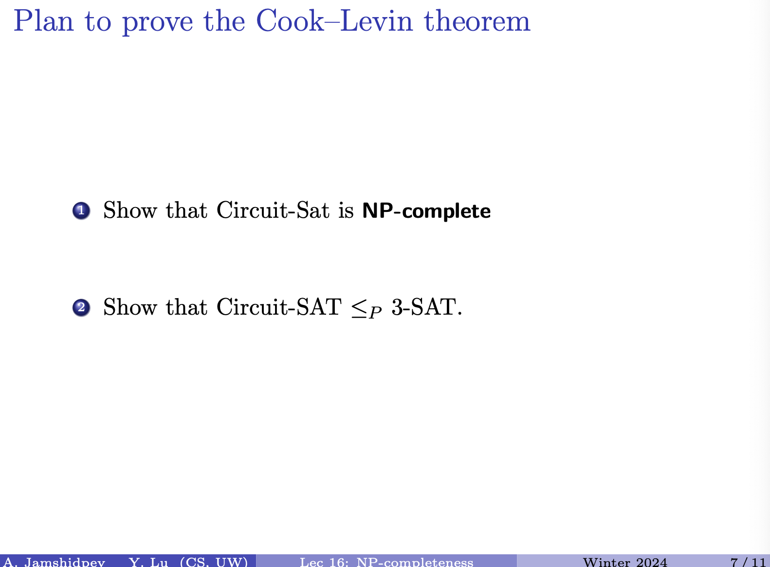
What’s the only thing we know about 3-SAT? There exist a polynomial time that we can provide a certificate.
- so in this case, we found that circuit-sat is NP complete, then if we show the circuit-sat is reducible to 3-sat, then all the np problems
- This is something different
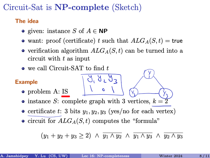
- We want and to not be in the set at the same time and the second clause checks that
Thu March 28: Goes back a couple slides and continues from slide 6/11
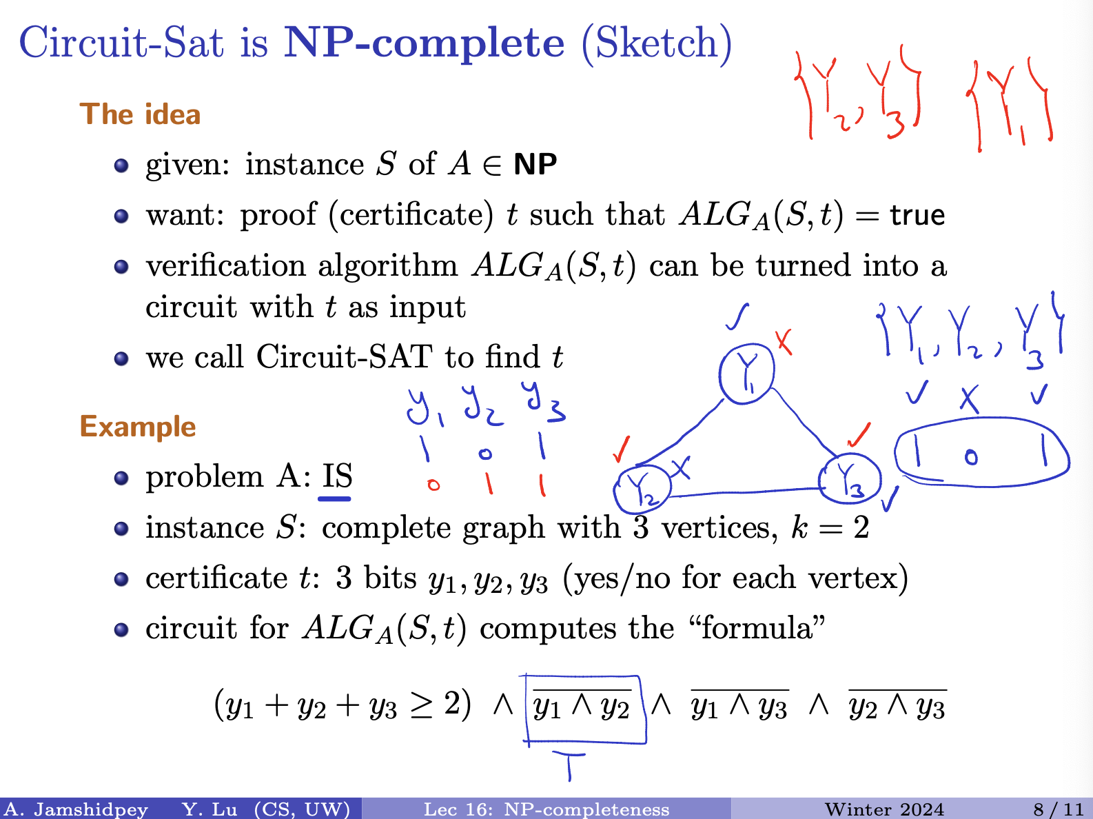
- Given a certificate ,
- Need to first check if the size . If so, it meets the first condition. Among y1 and y2, one of them at most can be in my set.
- If second condition is set to T, then initially, y1 and y2 are false.
- This is a no instance.
- What exactly is ?
Get an Instance of and IS, which is a graph + a integer (? I think) transform into a circuit. look at algorithm that verifies it. A circuit sat is np Use certificate and circuit for ALG that takes in and to compute a logical formula can be translated into a circuit, that would be my circuit
- From logic we know if and only [(p or not q) and (not p or q)]
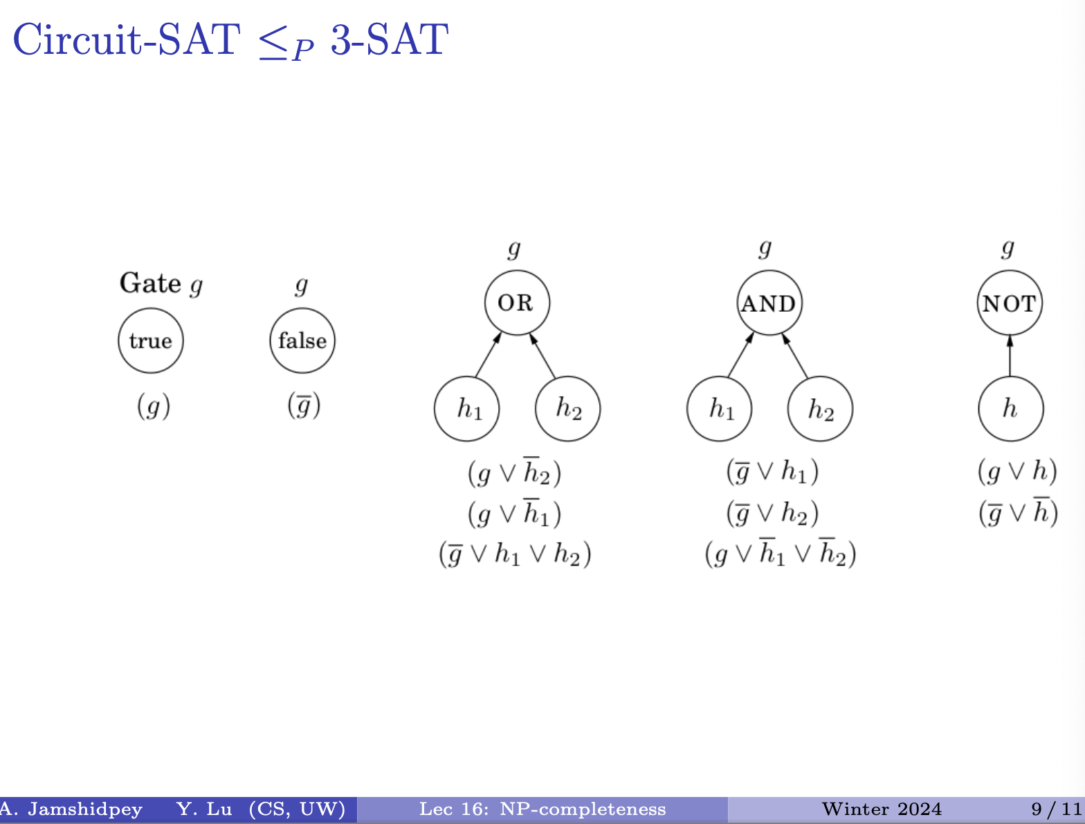
- We want to reduce Circuit-SAT into 3-SAT
- Note this slide doesn’t write conjunctions
Insert picture he drew (slide).
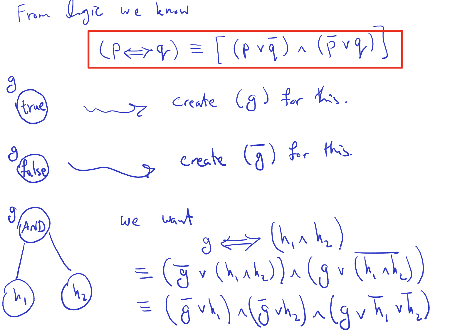
Insert the second slide he drew.
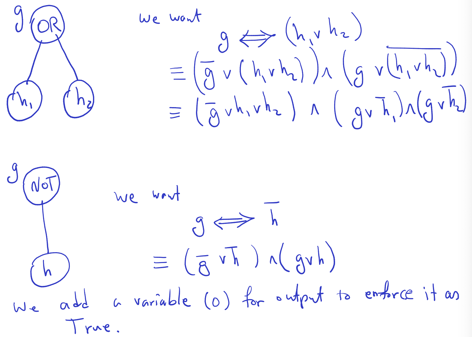
He is basically translating gates to CNF.
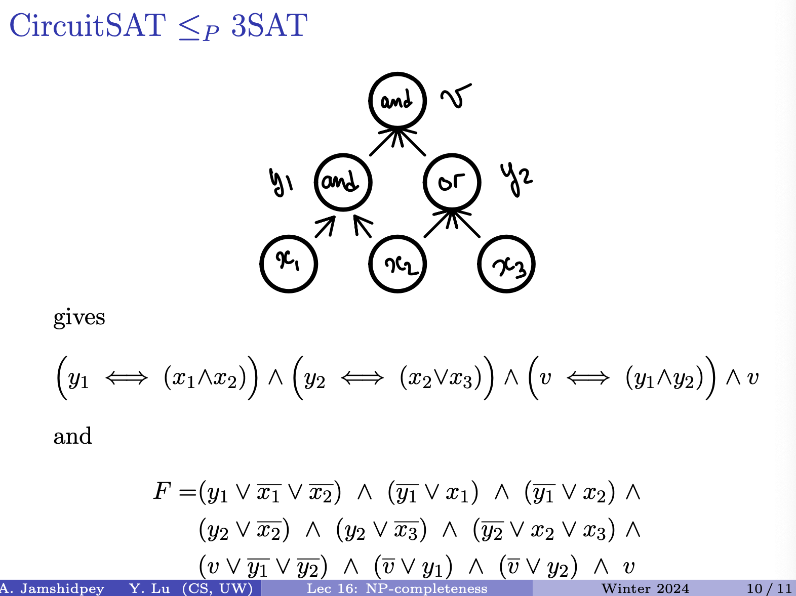
- write out the CNF
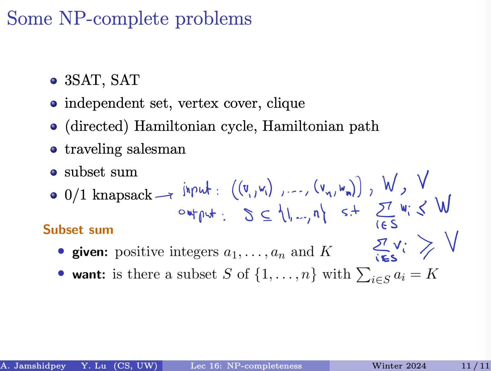
- (include annotated slide instead over here)
I’m very confused. Will need to review and understand this set of slides.
This module:
- prof takes care of hard part, we take care of easier part
- Next two sets of slides, you just need to remember the results for the final!!!!!!
- NP problems on the exam would be hard. Need to solve the np problem by yourself. And understand it
Tip, hint for future?
Hint for future: Which np complete prpblem to choose, usually when we don’t know which to start. Start with 3-SAT. Minimum set of requirements. And try to reduce 3-SAT to other problems.
Lecture 17 - NP-completeness Part 2
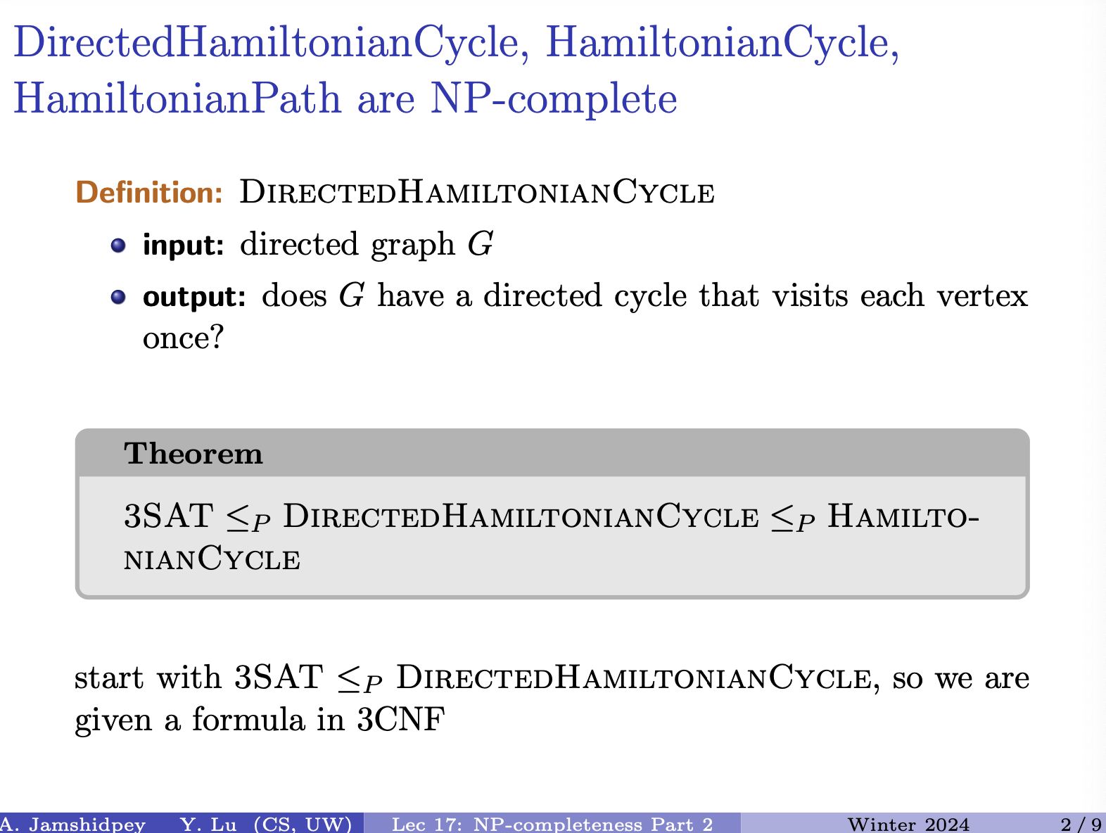
Starting the construction
Colour is not important, be able to recognize which part of the construction it is instead?
(include slide 3/9)
- For each clause, we create 3 nodes (2 sets?). Make sure that you go from left to right or from right to left. We enforce that there is no edges in between. So we have the option to explore from left to right or right to left, onto the next row or something.
- Create a source node and sink node
- He still want a hamiltonian cycle, so from t you can go to s
- Think about how he is constructing it, not why for now. 3 nodes per clause for each variable. are variables.
- Problem is to reduce 3-SAT to directed hamiltonian cycle
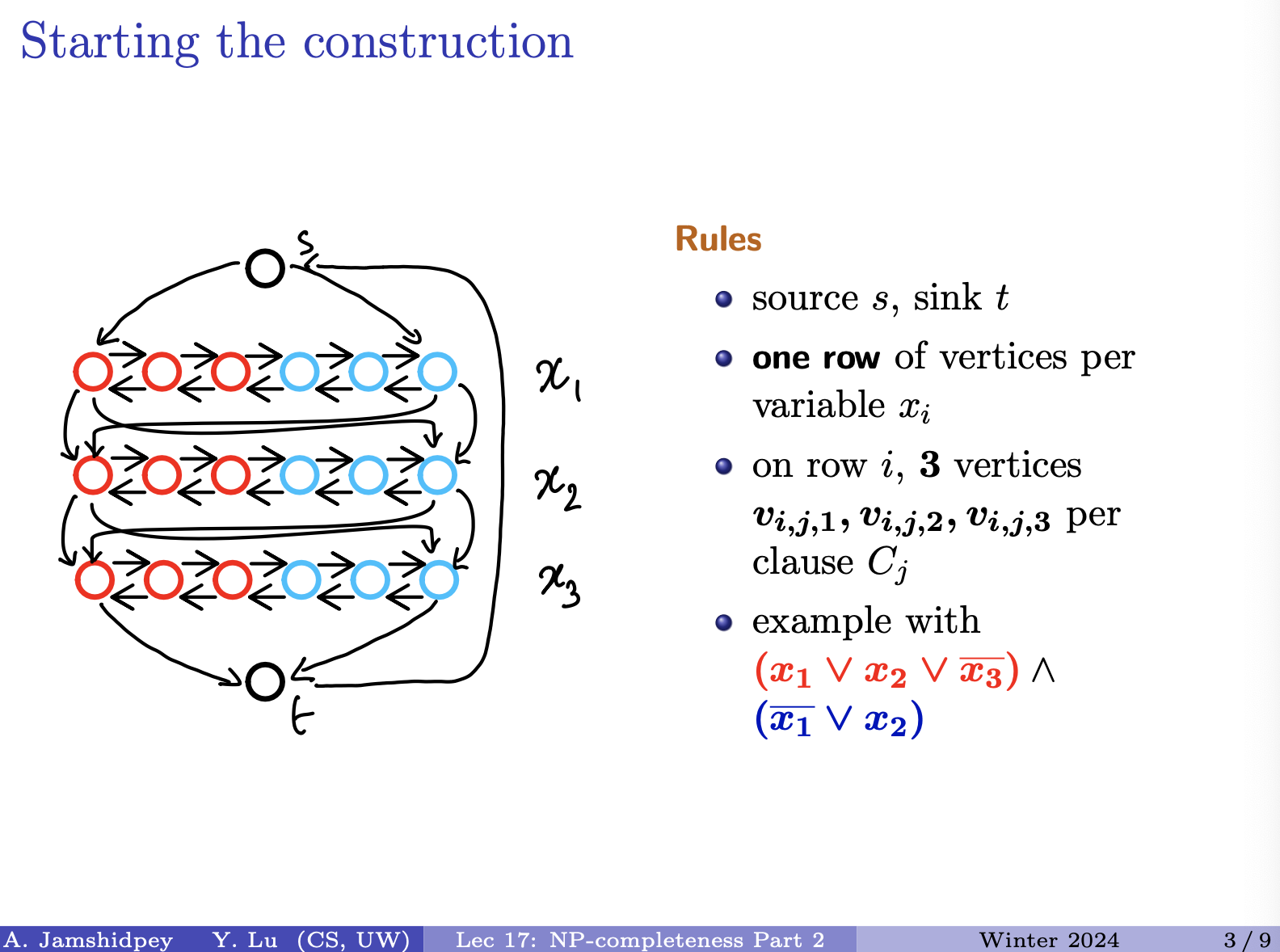
Observations:
- Do you see any hamiltonian cycles here? There exist hamiltonian cycles here. No matter which CNF given.
Write very short essay trying to explain what happened: try it
Learn efficient techniques. Learn how to learn more efficiently.
Tue April 2
Didn’t attend. Ask for notes. Bless mattloulou.todo
Thu April 4
Started Lecture 18.
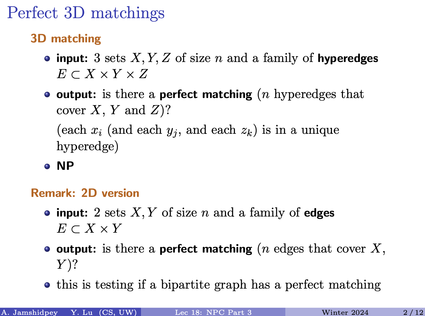
- sets are disjoint
- include his drawings
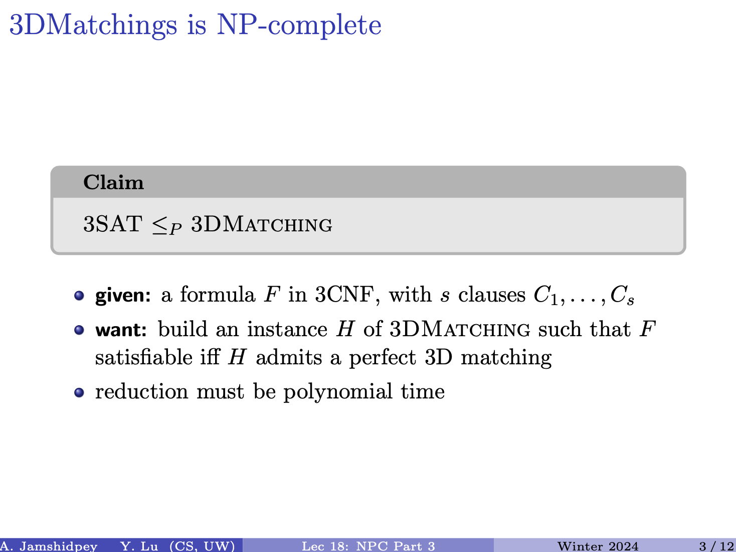
- Trying to form a gadget? We have a 3-SAT problem that we want to perform reduction. For each variable, we want to create a gadget.
- Line of vertices per variable. Lines of nodes he was creating for the Hamiltonian cycle thing in previous lecture probably.
- Include what he drew again.
- Encode true and false depending on the moving direction (left to right or vice versa). Purpose of last lecture.
- CNF is satisfiable if and only if it has perfect matching??
- n and s are input sizes?
- Include the drawing (aka two eggs)
- If you can solve B you can solve A
- Doesn’t care if he has injective map or … something else, don’t care direction from B to A. The two directions bottom right. yes instance
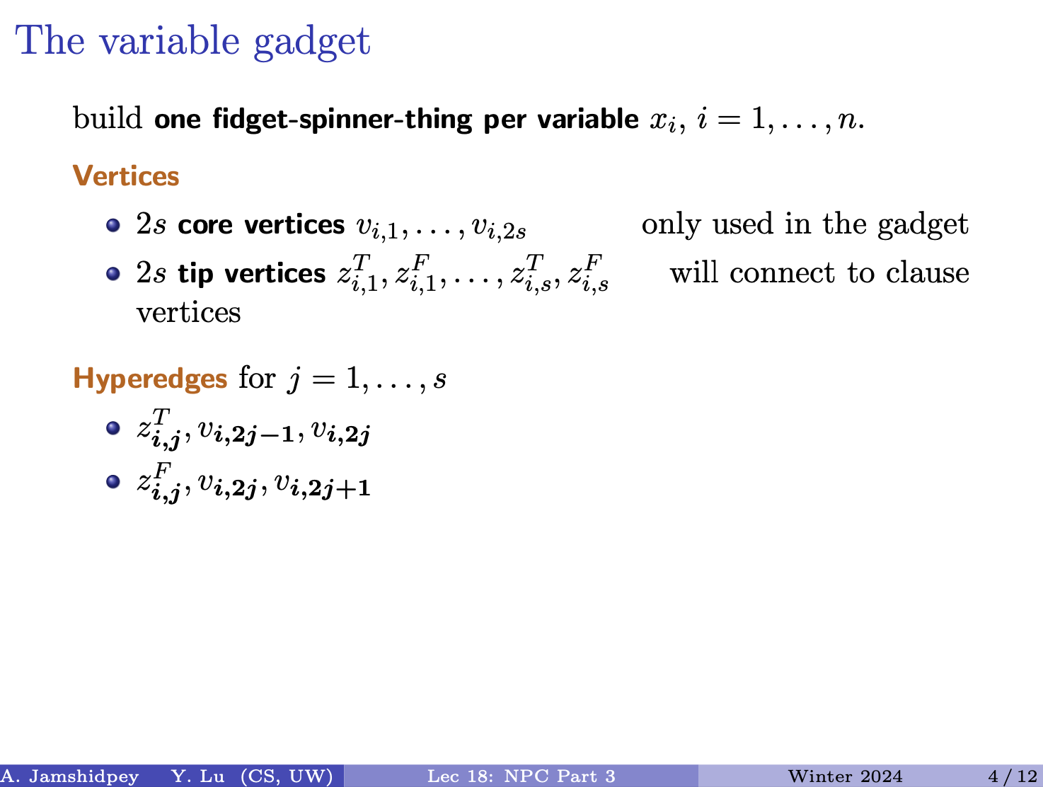
- do this per variable. we have s clauses.
- per clause we create two nodes (core vertices?) first number referring to variable, t version and y version?
- z, odd in x, even in y
- hypreedges: he drew 4 weird doritos that represents the fidget spinner gadget

- how do you pick hyperedges? from the total construction
- 2 ways
- take all hyperedges including t version or the false one
- he picks the top one on the left. can’t take left and right because they share nodes. Then he can only choose the the bottom one.
- 2 ways
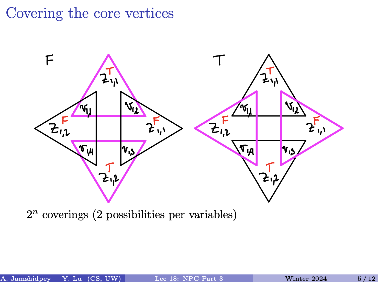
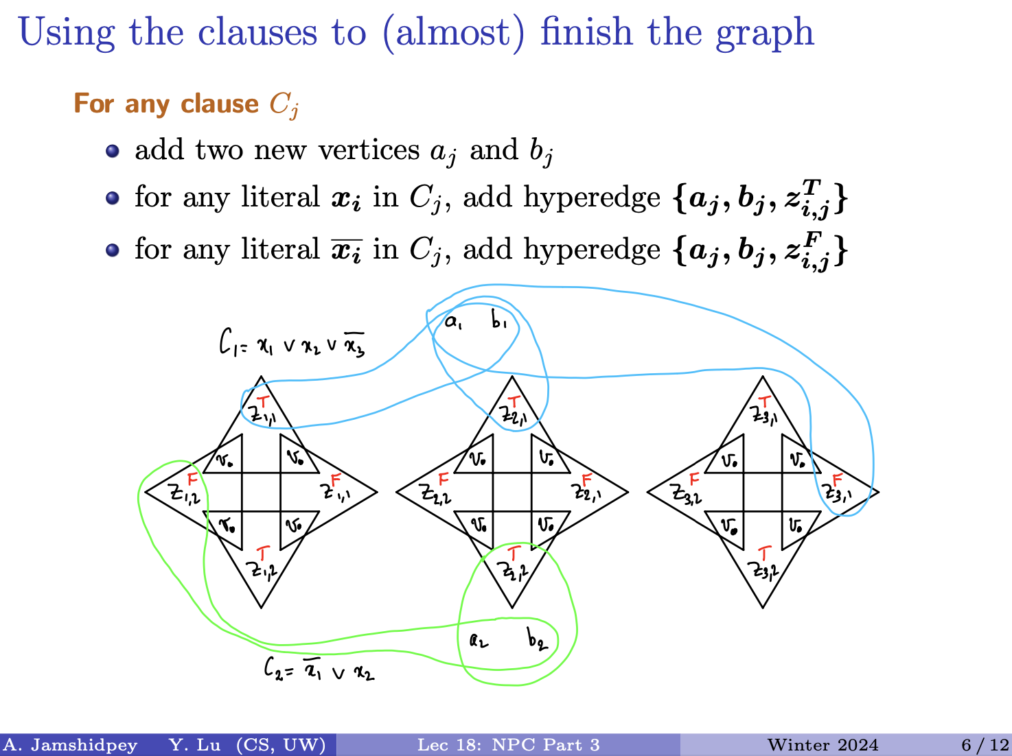
- T version of the tip to a1 and b1
- If i have negation of something. connect a1 b1 to the F version.
- x1 and x2 and x3 are set to F.
- We can say one thing, does these True assignment satisfy my assignment?
- Yes, we have a true assignment that satisfy my CNF.
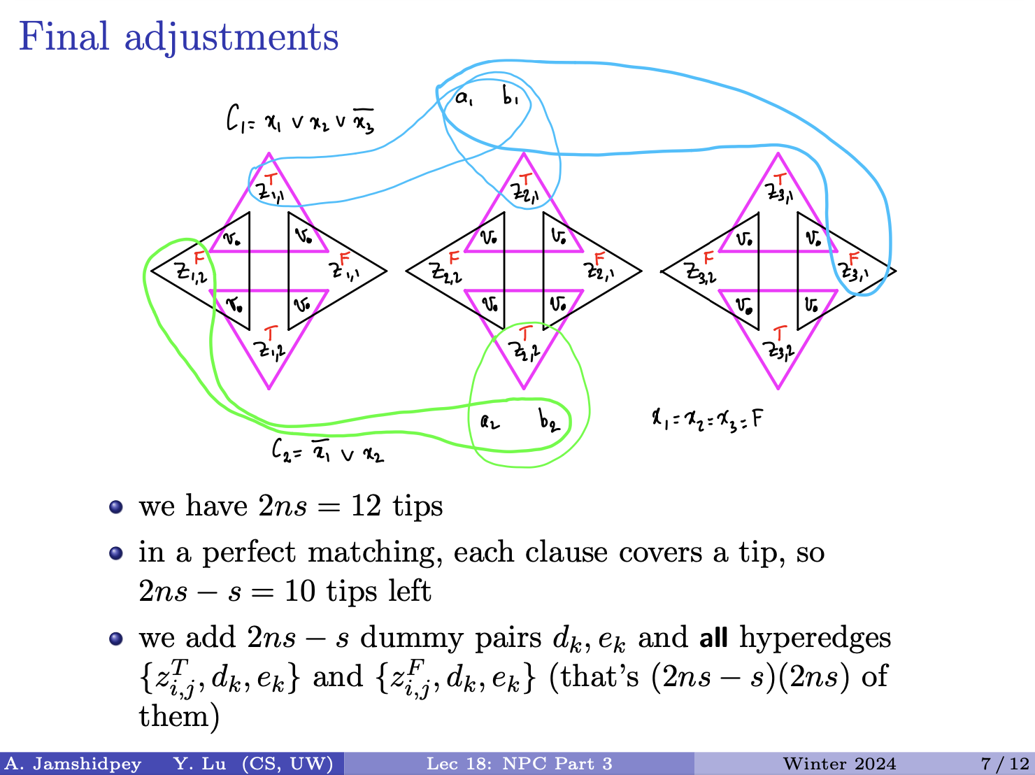
- C1: x3 is the one causing something
- C2: x1 is the one making sure
- There are tips that are not covered. So we need more vertices!!!!!!!!!!
- For each of these tips, we need to figure out how many are left. Total is 2ns = 12 tips
- s of them are covered for sure.
- 10 tips left at most not picked can be calculated using 2ns-s = 10. This is the upper bound.
- We can create a dummy vertices for something…
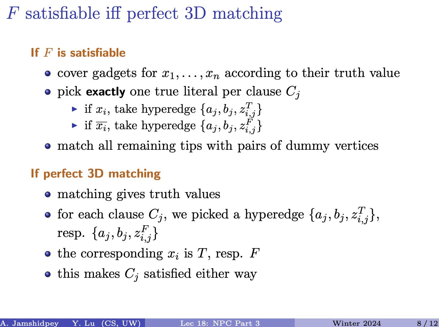
- make sure to pick exactly one! per clause
- so apparently we do have perfect matching
- Now from the other direction: they satisfy too. Just read the bullet points.
todo go home. He is not going to ask any proof. Good to understand the results.
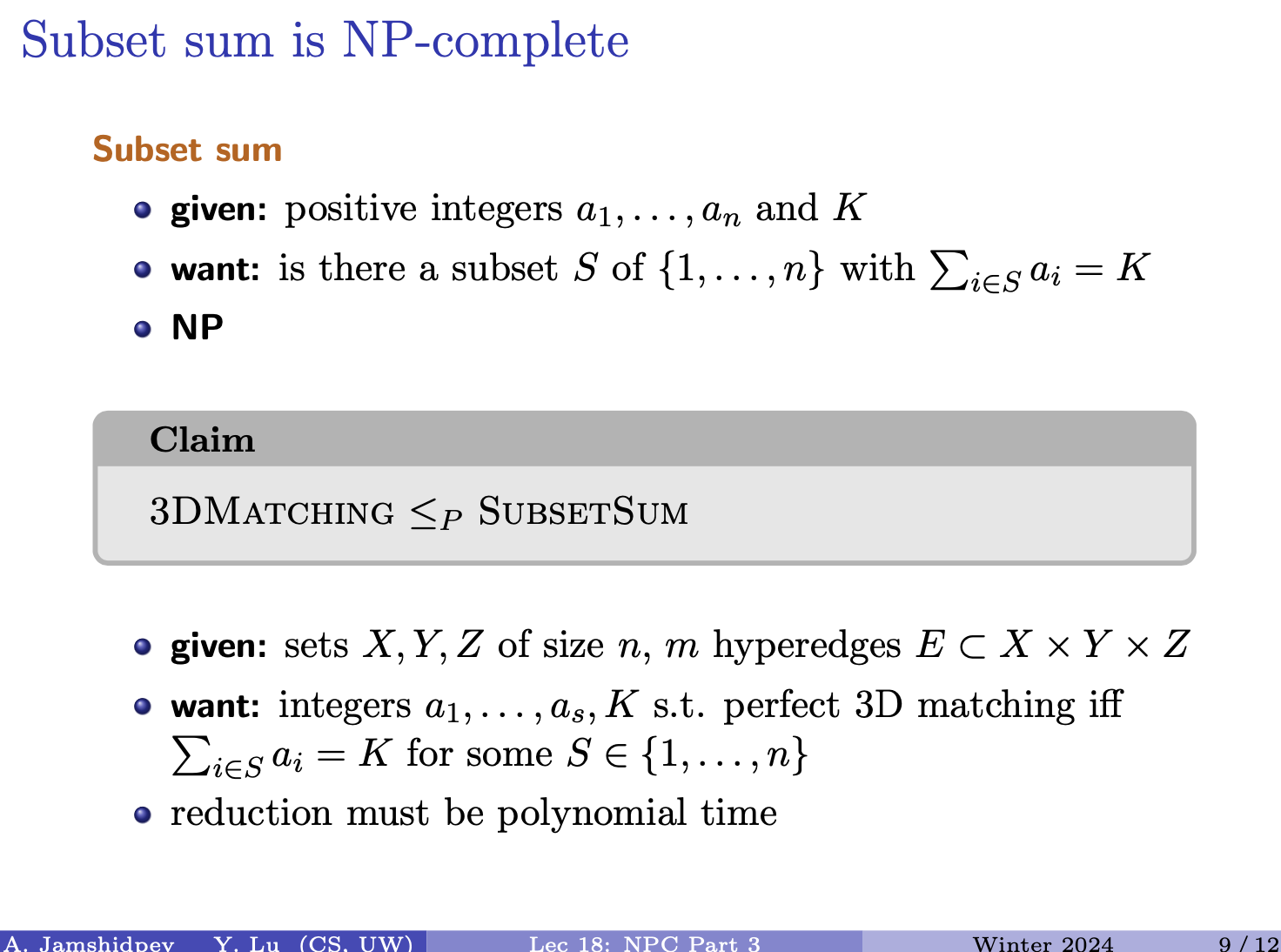
- 3D matching is in NP. Certificate is a potential solution. Algorithm checks if we visit every single edge in the hyperedge exactly once. Can be done in poly-time.
- certificate is a subset of these: in the slide.
- Now is it NP-Complete
Include his drawing
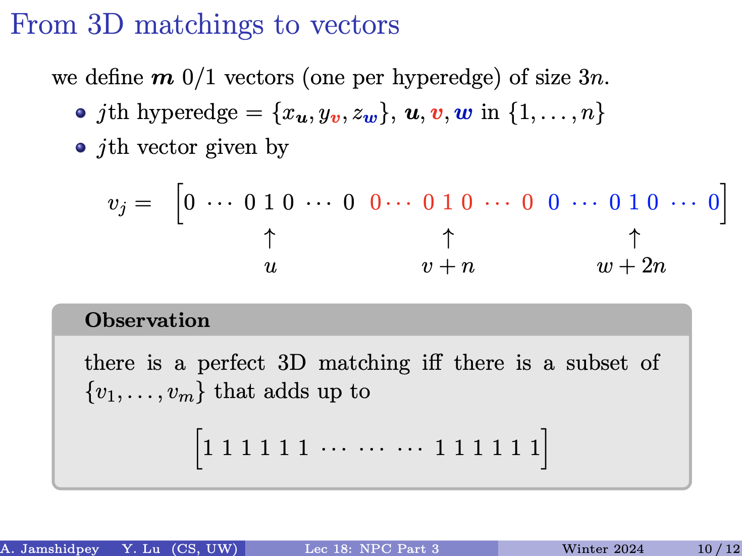
- must be true, only way to get 1, is to get a v1 in that position.
- We are picking some of these vectors
- If we have a 3D matching we are covering every vertex exactly once.
- These are not numbers, but they are vectors so far.
- In CS240, we saw that we can transform vector to number?
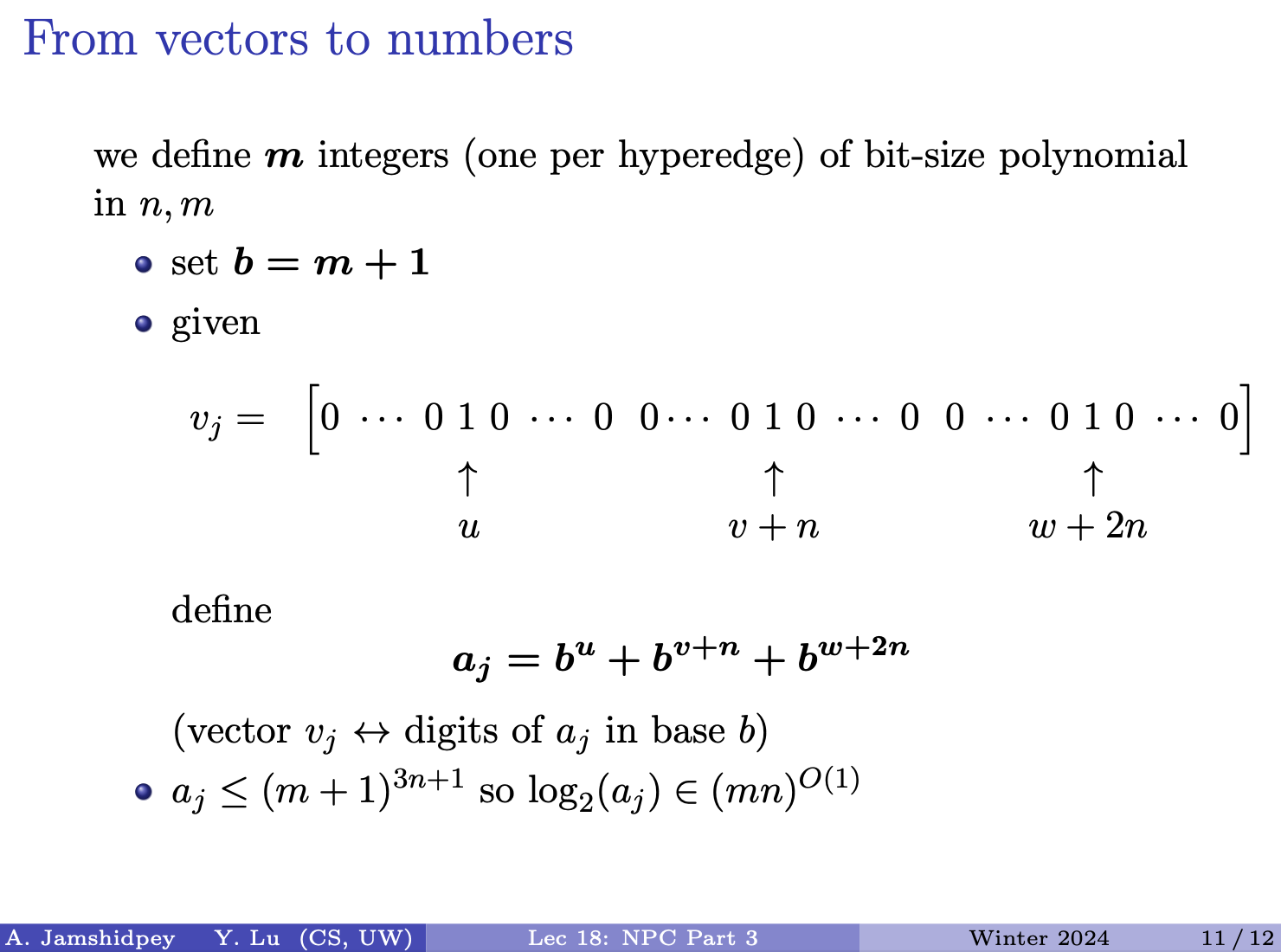
- choose base b to be m + 1. (for a reason)
- m is the number of hyperedges.
- so far for each vector, we create a number. Translate hyperedges to numbers. Forming a vector, converting to a number are both polynomial time.
- How large can be? Having everything as 1.
- The formula at the end: (m+1)^3n+1 will always be larger. Bounded by it.
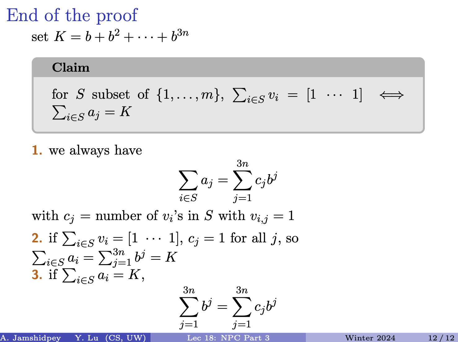
- What is K
- If we have with cj =number of vi’s in S with vi,j =1
- If this equality holds, then the later ones are easier to see.
- Remember base is m+1 (need to be)
- It is possible to choose m vectors and the sum is 1. So we make sure of s
The End. He showed this kung fu panda clip with master oogway and shifu.